

9. Physical Modeling
301
Where, p — mass density of water; g — gravitational accélération; h —
depth of water in the flume; H — wave height; T — Wave period; Bs —
Width of the structure, D
diameter of the végétation;
— diameter
at the root of the végétation, BG
width of green belt; fi — frequency of
first mode of the végétal stem; l — height of the végétation; SP — centre
to centre spacing between végétation; E — modulus of plant stifïness; L —
Wave length; (3 — Beach slope; Ru — Run-up; Vf — Flow velocity. The h
refers to, hs — depth of water at the toe of the structure; havg — average
depth of water on the up-stream and downstream of flow in open channel.
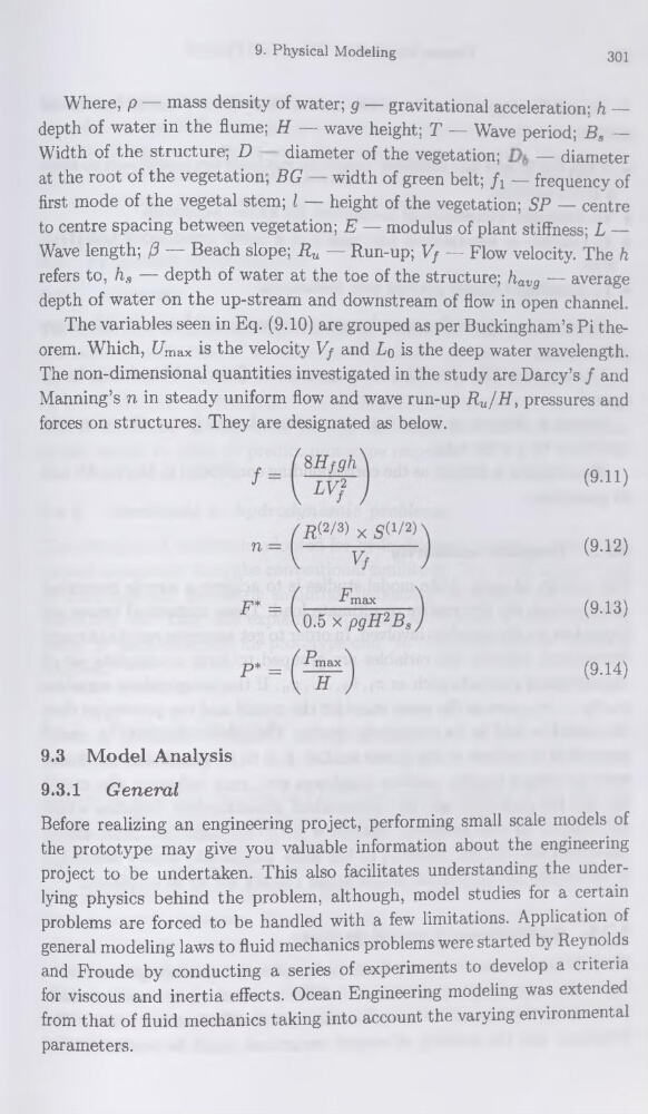
The variables seen in Eq. (9.10) are grouped as per Buckingham’s Pi theorem. Which, Umax is the velocity Vf and Lq is the deep water wavelength.
The non-dimensional quantifies investigated in the study are Darcy’s f and
Manning’s n in steady uniform flow and wave run-up Ru/H, pressures and
forces on structures. They are designated as below.
(9.11)
(9-12)
(9.13)
(9-14)
9.3 Model Analysis
9.3.1 General
Before realizing an engineering project, performing small scale models of
the prototype may give you valuable information about the engineering
Project to be undertaken. This also facilitâtes understanding the underlying physics behind the problem, although, model studies for a certain
problems are forced to be handled with a few limitations. Application of
general modeling laws to fluid mechanics problems were started by Reynolds
and Froude by conducting a sériés of experiments to develop a criteria
for viscous and inertia effects. Océan Engineering modeling was extended
from that of fluid mechanics taking into account the varying environmental
parameters.
301
Where, p — mass density of water; g — gravitational accélération; h —
depth of water in the flume; H — wave height; T — Wave period; Bs —
Width of the structure, D
diameter of the végétation;
— diameter
at the root of the végétation, BG
width of green belt; fi — frequency of
first mode of the végétal stem; l — height of the végétation; SP — centre
to centre spacing between végétation; E — modulus of plant stifïness; L —
Wave length; (3 — Beach slope; Ru — Run-up; Vf — Flow velocity. The h
refers to, hs — depth of water at the toe of the structure; havg — average
depth of water on the up-stream and downstream of flow in open channel.
The variables seen in Eq. (9.10) are grouped as per Buckingham’s Pi theorem. Which, Umax is the velocity Vf and Lq is the deep water wavelength.
The non-dimensional quantifies investigated in the study are Darcy’s f and
Manning’s n in steady uniform flow and wave run-up Ru/H, pressures and
forces on structures. They are designated as below.
(9.11)
(9-12)
(9.13)
(9-14)
9.3 Model Analysis
9.3.1 General
Before realizing an engineering project, performing small scale models of
the prototype may give you valuable information about the engineering
Project to be undertaken. This also facilitâtes understanding the underlying physics behind the problem, although, model studies for a certain
problems are forced to be handled with a few limitations. Application of
general modeling laws to fluid mechanics problems were started by Reynolds
and Froude by conducting a sériés of experiments to develop a criteria
for viscous and inertia effects. Océan Engineering modeling was extended
from that of fluid mechanics taking into account the varying environmental
parameters.