

300
Coastal Engineering: Theory and Practice
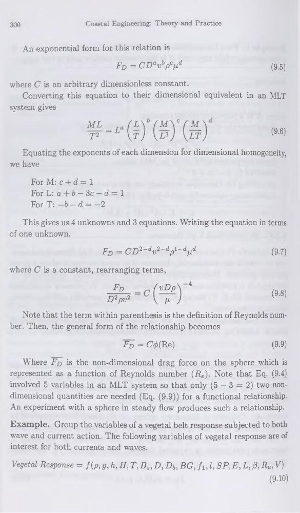
An exponential form for this relation is
Fd = CD°
where C is an arbitrary dimensionless constant.
Converting this équation to their dimensional équivalent in an MLT
System gives
ML _
(L\h (M\c ( M_\
T2 ~L \t) \L*) \Lt)
(9-6)
Equating the exponents of each dimension for dimensional homogeneity,
we hâve
For M: c + d = 1
For L: a + b — 3c — d = 1
For T: -b - d = -2
This gives us 4 unknowns and 3 équations. Writing the équation in terms
of one unknown,
Fd = CD2~dv2~dp1~dpd
(9.7)
where C* is a constant, rearranging terms,
Fp _
/vDp\ 4
D2pv2
y p J
(9-8)
Note that the term within parenthesis is the définition of Reynolds number. Then, the general form of the relationship becomes
Fp = C0(Re)
(9.9)
Where Fp is the non-dimensional drag force on the sphere which is
represented as a function of Reynolds number (Re). Note that Eq. (9.4)
involved 5 variables in an MLT System so that only (5 — 3 = 2) two nondimensional quantities are needed (Eq. (9.9)) for a functional relationship.
An experiment with a sphere in steady flow produces such a relationship.
Example. Group the variables of a végétal belt response subjected to both
wave and current action. The following variables of végétal response are of
interest for both currents and waves.
Végétal Response = f(p, g, h, H, T, Bs, D, Db, BG, fa.l, SP. E. L, (3, Ru, V)
(9.10)
Coastal Engineering: Theory and Practice
An exponential form for this relation is
Fd = CD°
where C is an arbitrary dimensionless constant.
Converting this équation to their dimensional équivalent in an MLT
System gives
ML _
(L\h (M\c ( M_\
T2 ~L \t) \L*) \Lt)
(9-6)
Equating the exponents of each dimension for dimensional homogeneity,
we hâve
For M: c + d = 1
For L: a + b — 3c — d = 1
For T: -b - d = -2
This gives us 4 unknowns and 3 équations. Writing the équation in terms
of one unknown,
Fd = CD2~dv2~dp1~dpd
(9.7)
where C* is a constant, rearranging terms,
Fp _
/vDp\ 4
D2pv2
y p J
(9-8)
Note that the term within parenthesis is the définition of Reynolds number. Then, the general form of the relationship becomes
Fp = C0(Re)
(9.9)
Where Fp is the non-dimensional drag force on the sphere which is
represented as a function of Reynolds number (Re). Note that Eq. (9.4)
involved 5 variables in an MLT System so that only (5 — 3 = 2) two nondimensional quantities are needed (Eq. (9.9)) for a functional relationship.
An experiment with a sphere in steady flow produces such a relationship.
Example. Group the variables of a végétal belt response subjected to both
wave and current action. The following variables of végétal response are of
interest for both currents and waves.
Végétal Response = f(p, g, h, H, T, Bs, D, Db, BG, fa.l, SP. E. L, (3, Ru, V)
(9.10)