

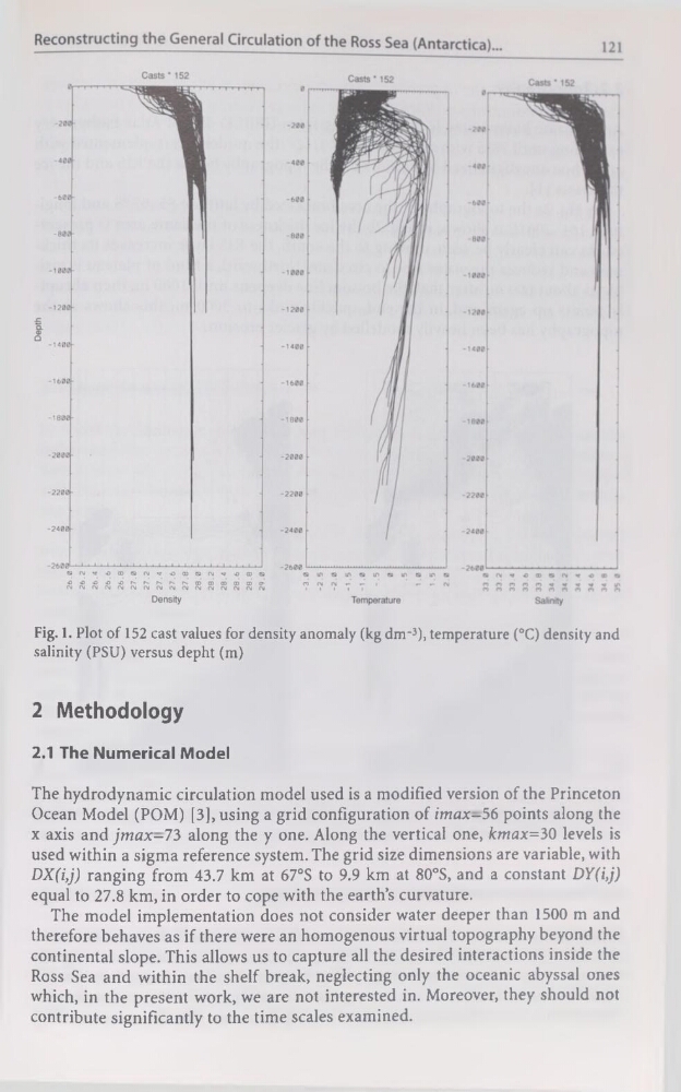
Fig. 1. Plot of 152 cast values for density anomaly (kg dm-3), température (°C) density and
salinity (PSU) versus depht (m)
2 Methodology
2.1 The Numerical Mode!
The hydrodynamic circulation model used is a modified version of the Princeton
Océan Model (POM) [3], using a grid configuration of imax-56 points along the
x axis and jmax-73 along the y one. Along the vertical one, kmax=30 levels is
used within a sigma reference System. The grid size dimensions are variable, with
DX(i,j) ranging from 43.7 km at 67°S to 9.9 km at 80°S, and a constant DY(i,j)
equal to 27.8 km, in order to cope with the earth’s curvature.
The model implémentation does not consider water deeper than 1500 m and
therefore behaves as if there were an homogenous virtual topography beyond the
continental slope. This allows us to capture ail the desired interactions inside the
Ross Sea and within the shelf break, neglecting only the oceanic abyssal ones
which, in the présent work, we are not interested in. Moreover, they should not
contribute significantly to the time scales examined.
salinity (PSU) versus depht (m)
2 Methodology
2.1 The Numerical Mode!
The hydrodynamic circulation model used is a modified version of the Princeton
Océan Model (POM) [3], using a grid configuration of imax-56 points along the
x axis and jmax-73 along the y one. Along the vertical one, kmax=30 levels is
used within a sigma reference System. The grid size dimensions are variable, with
DX(i,j) ranging from 43.7 km at 67°S to 9.9 km at 80°S, and a constant DY(i,j)
equal to 27.8 km, in order to cope with the earth’s curvature.
The model implémentation does not consider water deeper than 1500 m and
therefore behaves as if there were an homogenous virtual topography beyond the
continental slope. This allows us to capture ail the desired interactions inside the
Ross Sea and within the shelf break, neglecting only the oceanic abyssal ones
which, in the présent work, we are not interested in. Moreover, they should not
contribute significantly to the time scales examined.