

70 Computational Modelling in Hydraulic and Coastal Engineering
4.3.2 Momentum equation for water hammer
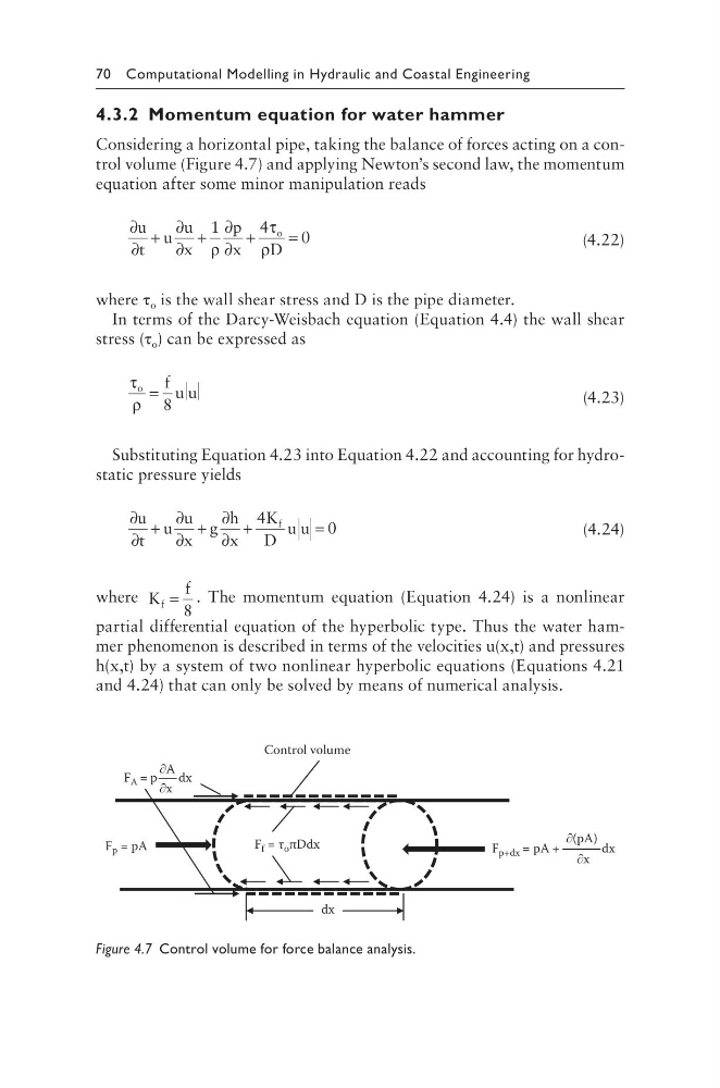
Considering a horizontal pipe, taking the balance of forces acting on a control volume (Figure 4.7) and applying Newton’s second law, the momentum
equation after some minor manipulation reads
∂
∂
+
∂
∂
+
∂
∂
+
=
u
t
u
u
x
p
x
D
o
1
4
0
ρ
τ
ρ
(4.22)
where τ o is the wall shear stress and D is the pipe diameter.
In terms of the Darcy-Weisbach equation (Equation 4.4) the wall shear
stress (τ o ) can be expressed as
τ
ρ
o
f u u
= 8
(4.23)
Substituting Equation 4.23 into Equation 4.22 and accounting for hydrostatic pressure yields
∂
∂
+
∂
∂
+
∂
∂
+
=
u
t
u
u
x
g
h
x
K
D
u u
f
4
0
(4.24)
where K
f
f = 8
. The momentum equation (Equation 4.24) is a nonlinear
partial differential equation of the hyperbolic type. Thus the water hammer phenomenon is described in terms of the velocities u(x,t) and pressures
h(x,t) by a system of two nonlinear hyperbolic equations (Equations 4.21
and 4.24) that can only be solved by means of numerical analysis.
F p+dx =
∂(pA)
pA +
d x
∂x
F p = pA
dx
Control volume
F f = τ o πDdx
F A =
∂A
p
dx
∂x
Figure 4.7 Control volume for force balance analysis.
4.3.2 Momentum equation for water hammer
Considering a horizontal pipe, taking the balance of forces acting on a control volume (Figure 4.7) and applying Newton’s second law, the momentum
equation after some minor manipulation reads
∂
∂
+
∂
∂
+
∂
∂
+
=
u
t
u
u
x
p
x
D
o
1
4
0
ρ
τ
ρ
(4.22)
where τ o is the wall shear stress and D is the pipe diameter.
In terms of the Darcy-Weisbach equation (Equation 4.4) the wall shear
stress (τ o ) can be expressed as
τ
ρ
o
f u u
= 8
(4.23)
Substituting Equation 4.23 into Equation 4.22 and accounting for hydrostatic pressure yields
∂
∂
+
∂
∂
+
∂
∂
+
=
u
t
u
u
x
g
h
x
K
D
u u
f
4
0
(4.24)
where K
f
f = 8
. The momentum equation (Equation 4.24) is a nonlinear
partial differential equation of the hyperbolic type. Thus the water hammer phenomenon is described in terms of the velocities u(x,t) and pressures
h(x,t) by a system of two nonlinear hyperbolic equations (Equations 4.21
and 4.24) that can only be solved by means of numerical analysis.
F p+dx =
∂(pA)
pA +
d x
∂x
F p = pA
dx
Control volume
F f = τ o πDdx
F A =
∂A
p
dx
∂x
Figure 4.7 Control volume for force balance analysis.