

Common partial differential equations of computational hydraulics 41
Given the value of the diffusion coefficient N and the space discretization
step Δx, the time step Δt has to be selected in compliance to the inequality
Equation 3.24. Otherwise the numerical computations would overflow.
3.3.2.2 Crank-Nicolson numerical scheme
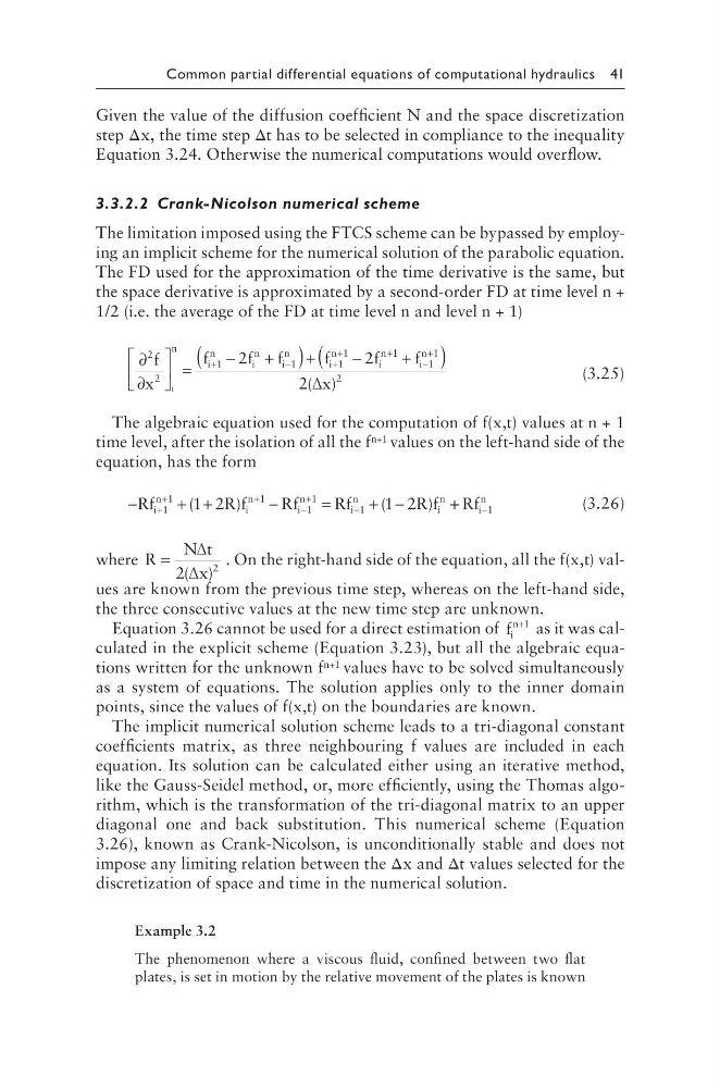
The limitation imposed using the FTCS scheme can be bypassed by employing an implicit scheme for the numerical solution of the parabolic equation.
The FD used for the approximation of the time derivative is the same, but
the space derivative is approximated by a second-order FD at time level n +
1/2 (i.e. the average of the FD at time level n and level n + 1)
∂
∂
=
−
+
(
)+ −
+
−
+
+
+
2
2
1
1
1
1
2
2
f
x
f
f f
f
f
i
n
i
n
i
n
i
n
i
n
i
n 1 1
1
1
2
2
+
(
)
−
+
f
x
i
n
( )
∆
(3.25)
The algebraic equation used for the computation of f(x,t) values at n + 1
time level, after the isolation of all the f n+1 values on the left-hand side of the
equation, has the form
−
+ +
−
=
+ −
+
+
+
−
+
+
Rf
R f
Rf
Rf
R f
i
n
i
n
i
n
i
n
i
n
1
1
1
1
1
1
1 2
1 2
(
)
(
) + + −
Rf i
n
1
(3.26)
where R
N t
x
=
∆
∆
2
2
( )
. On the right-hand side of the equation, all the f(x,t) values are known from the previous time step, whereas on the left-hand side,
the three consecutive values at the new time step are unknown.
Equation 3.26 cannot be used for a direct estimation of f i
n+1
as it was calculated in the explicit scheme (Equation 3.23), but all the algebraic equations written for the unknown f n+1 values have to be solved simultaneously
as a system of equations. The solution applies only to the inner domain
points, since the values of f(x,t) on the boundaries are known.
The implicit numerical solution scheme leads to a tri-diagonal constant
coefficients matrix, as three neighbouring f values are included in each
equation. Its solution can be calculated either using an iterative method,
like the Gauss-Seidel method, or, more efficiently, using the Thomas algorithm, which is the transformation of the tri-diagonal matrix to an upper
diagonal one and back substitution. This numerical scheme (Equation
3.26), known as Crank-Nicolson, is unconditionally stable and does not
impose any limiting relation between the Δx and Δt values selected for the
discretization of space and time in the numerical solution.
Example 3.2
The phenomenon where a viscous fluid, confined between two flat
plates, is set in motion by the relative movement of the plates is known
Given the value of the diffusion coefficient N and the space discretization
step Δx, the time step Δt has to be selected in compliance to the inequality
Equation 3.24. Otherwise the numerical computations would overflow.
3.3.2.2 Crank-Nicolson numerical scheme
The limitation imposed using the FTCS scheme can be bypassed by employing an implicit scheme for the numerical solution of the parabolic equation.
The FD used for the approximation of the time derivative is the same, but
the space derivative is approximated by a second-order FD at time level n +
1/2 (i.e. the average of the FD at time level n and level n + 1)
∂
∂
=
−
+
(
)+ −
+
−
+
+
+
2
2
1
1
1
1
2
2
f
x
f
f f
f
f
i
n
i
n
i
n
i
n
i
n
i
n 1 1
1
1
2
2
+
(
)
−
+
f
x
i
n
( )
∆
(3.25)
The algebraic equation used for the computation of f(x,t) values at n + 1
time level, after the isolation of all the f n+1 values on the left-hand side of the
equation, has the form
−
+ +
−
=
+ −
+
+
+
−
+
+
Rf
R f
Rf
Rf
R f
i
n
i
n
i
n
i
n
i
n
1
1
1
1
1
1
1 2
1 2
(
)
(
) + + −
Rf i
n
1
(3.26)
where R
N t
x
=
∆
∆
2
2
( )
. On the right-hand side of the equation, all the f(x,t) values are known from the previous time step, whereas on the left-hand side,
the three consecutive values at the new time step are unknown.
Equation 3.26 cannot be used for a direct estimation of f i
n+1
as it was calculated in the explicit scheme (Equation 3.23), but all the algebraic equations written for the unknown f n+1 values have to be solved simultaneously
as a system of equations. The solution applies only to the inner domain
points, since the values of f(x,t) on the boundaries are known.
The implicit numerical solution scheme leads to a tri-diagonal constant
coefficients matrix, as three neighbouring f values are included in each
equation. Its solution can be calculated either using an iterative method,
like the Gauss-Seidel method, or, more efficiently, using the Thomas algorithm, which is the transformation of the tri-diagonal matrix to an upper
diagonal one and back substitution. This numerical scheme (Equation
3.26), known as Crank-Nicolson, is unconditionally stable and does not
impose any limiting relation between the Δx and Δt values selected for the
discretization of space and time in the numerical solution.
Example 3.2
The phenomenon where a viscous fluid, confined between two flat
plates, is set in motion by the relative movement of the plates is known