

40 Computational Modelling in Hydraulic and Coastal Engineering
Then, after some simple rearrangement, the algebraic equation that approximates the differential equation (Equation 3.4) at point (i,n) reads
f
f
N
t
x
f
f
f
i
n
i
n
i
n
i
n
i
n
+
+
−
= +
−
+
(
)
1
2
1
1
2
∆
∆
( )
(3.23)
This numerical algorithm is explicit and is known as the FTCS scheme. The
numerical solution algorithm is organized as follows.
Note that in the above equation N is the diffusion coefficient, different
from the upper limit N of the index n.
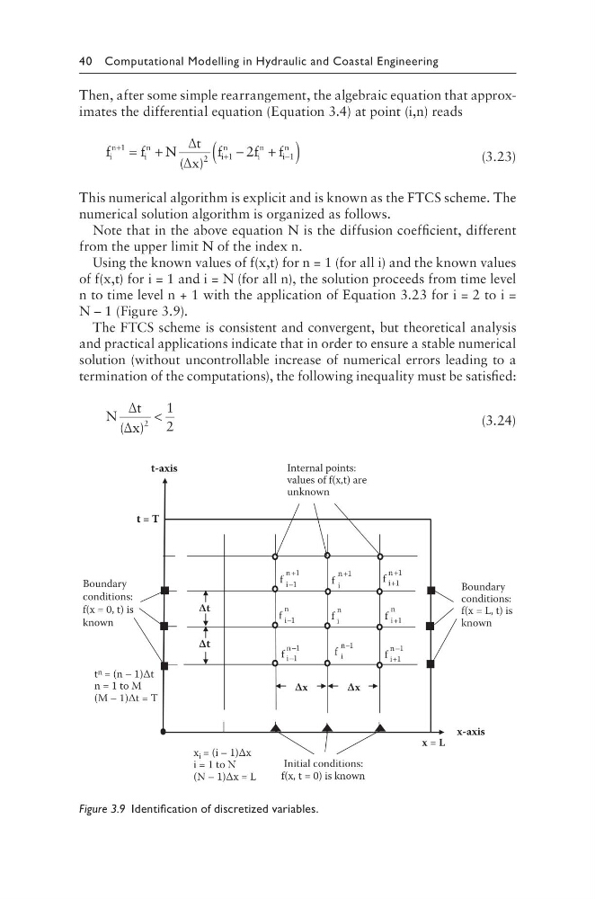
Using the known values of f(x,t) for n = 1 (for all i) and the known values
of f(x,t) for i = 1 and i = N (for all n), the solution proceeds from time level
n to time level n + 1 with the application of Equation 3.23 for i = 2 to i =
N – 1 (Figure 3.9).
The FTCS scheme is consistent and convergent, but theoretical analysis
and practical applications indicate that in order to ensure a stable numerical
solution (without uncontrollable increase of numerical errors leading to a
termination of the computations), the following inequality must be satisfied:
N
t
x
∆
∆
( )
2
1
2
<
(3.24)
n–1
i
f
n
i+1
f
n
i
f
n
i–1
f
n–1
i–1
f
n–1
i+1
f
n+1
i+1
f
n+1
i
f
n+1
i–1
f
t n = (n – 1)Δt
n = 1 to M
(M – 1)Δt = T
Δt
Δt
t = T
x = L
x-axis
Internal points:
values of f(x,t) are
unknown
t-axis
Δx
Boundary
conditions:
f(x = 0, t) is
known
Boundary
conditions:
f(x = L, t) is
known
Initial conditions:
f(x, t = 0) is known
Δx
x i = (i – 1)Δx
i = 1 to N
(N – 1)Δx = L
Figure 3.9 Identification of discretized variables.
Then, after some simple rearrangement, the algebraic equation that approximates the differential equation (Equation 3.4) at point (i,n) reads
f
f
N
t
x
f
f
f
i
n
i
n
i
n
i
n
i
n
+
+
−
= +
−
+
(
)
1
2
1
1
2
∆
∆
( )
(3.23)
This numerical algorithm is explicit and is known as the FTCS scheme. The
numerical solution algorithm is organized as follows.
Note that in the above equation N is the diffusion coefficient, different
from the upper limit N of the index n.
Using the known values of f(x,t) for n = 1 (for all i) and the known values
of f(x,t) for i = 1 and i = N (for all n), the solution proceeds from time level
n to time level n + 1 with the application of Equation 3.23 for i = 2 to i =
N – 1 (Figure 3.9).
The FTCS scheme is consistent and convergent, but theoretical analysis
and practical applications indicate that in order to ensure a stable numerical
solution (without uncontrollable increase of numerical errors leading to a
termination of the computations), the following inequality must be satisfied:
N
t
x
∆
∆
( )
2
1
2
<
(3.24)
n–1
i
f
n
i+1
f
n
i
f
n
i–1
f
n–1
i–1
f
n–1
i+1
f
n+1
i+1
f
n+1
i
f
n+1
i–1
f
t n = (n – 1)Δt
n = 1 to M
(M – 1)Δt = T
Δt
Δt
t = T
x = L
x-axis
Internal points:
values of f(x,t) are
unknown
t-axis
Δx
Boundary
conditions:
f(x = 0, t) is
known
Boundary
conditions:
f(x = L, t) is
known
Initial conditions:
f(x, t = 0) is known
Δx
x i = (i – 1)Δx
i = 1 to N
(N – 1)Δx = L
Figure 3.9 Identification of discretized variables.