

28 Computational Modelling in Hydraulic and Coastal Engineering
where φ is a known function. For φ = 0, the equation reduces to the wellknown Laplace equation. In physical terms Equation 3.3 represents the
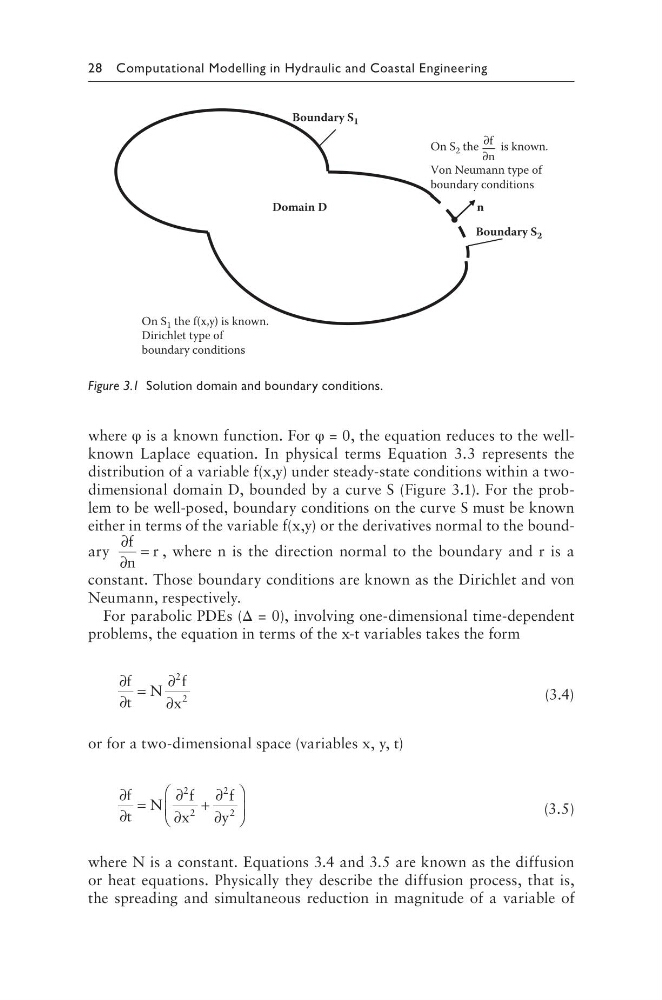
distribution of a variable f(x,y) under steady-state conditions within a twodimensional domain D, bounded by a curve S (Figure 3.1). For the problem to be well-posed, boundary conditions on the curve S must be known
either in terms of the variable f(x,y) or the derivatives normal to the boundary
∂
∂
=
f
n
r , where n is the direction normal to the boundary and r is a
constant. Those boundary conditions are known as the Dirichlet and von
Neumann, respectively.
For parabolic PDEs (Δ = 0), involving one-dimensional time-dependent
problems, the equation in terms of the x-t variables takes the form
∂
∂
=
∂
∂
f
t
N
f
x
2
2
(3.4)
or for a two-dimensional space (variables x, y, t)
∂
∂
=
∂
∂
+
∂
∂
f
t
N
f
x
f
y
2
2
2
2
(3.5)
where N is a constant. Equations 3.4 and 3.5 are known as the diffusion
or heat equations. Physically they describe the diffusion process, that is,
the spreading and simultaneous reduction in magnitude of a variable of
On S 2 the
∂f
∂n
is known.
Von Neumann type of
boundary conditions
On S 1 the f(x,y) is known.
Dirichlet type of
boundary conditions
Boundary S 1
Boundary S 2
n
Domain D
Figure 3.1 Solution domain and boundary conditions.
where φ is a known function. For φ = 0, the equation reduces to the wellknown Laplace equation. In physical terms Equation 3.3 represents the
distribution of a variable f(x,y) under steady-state conditions within a twodimensional domain D, bounded by a curve S (Figure 3.1). For the problem to be well-posed, boundary conditions on the curve S must be known
either in terms of the variable f(x,y) or the derivatives normal to the boundary
∂
∂
=
f
n
r , where n is the direction normal to the boundary and r is a
constant. Those boundary conditions are known as the Dirichlet and von
Neumann, respectively.
For parabolic PDEs (Δ = 0), involving one-dimensional time-dependent
problems, the equation in terms of the x-t variables takes the form
∂
∂
=
∂
∂
f
t
N
f
x
2
2
(3.4)
or for a two-dimensional space (variables x, y, t)
∂
∂
=
∂
∂
+
∂
∂
f
t
N
f
x
f
y
2
2
2
2
(3.5)
where N is a constant. Equations 3.4 and 3.5 are known as the diffusion
or heat equations. Physically they describe the diffusion process, that is,
the spreading and simultaneous reduction in magnitude of a variable of
On S 2 the
∂f
∂n
is known.
Von Neumann type of
boundary conditions
On S 1 the f(x,y) is known.
Dirichlet type of
boundary conditions
Boundary S 1
Boundary S 2
n
Domain D
Figure 3.1 Solution domain and boundary conditions.