

278 Computational Modelling in Hydraulic and Coastal Engineering
c
u
u
u u u
u
g
t
x
3
1
2
1
2
1 2
2
2
1
2
3
2
2
3
1
2
=
+
+
−
−
+
−
−
(
)
(
)
ζ ζ
∆
∆
( (
)
u
u S e
1
2
2
+
(9.103)
c
h
h
S x u
h
h
S x u
o
o
4
1
3
1
4
3
1
2
=
−
+
−
+
+
(
)
(
)
λ
λ
∆
∆
2 2
∆
∆
t
x
+
−
+ −
+
− +
2
1
8
1
1
8
4
3
1 1
1 2
2 1
λ
ζ
λ
ζ
ζ
∆
∆
x u
x u
u
(
)
8 8
2 2
λ
ζ
∆
∆
∆
x u
t
x
+3(ζ 1 + 2ζ 2 )
(9.104)
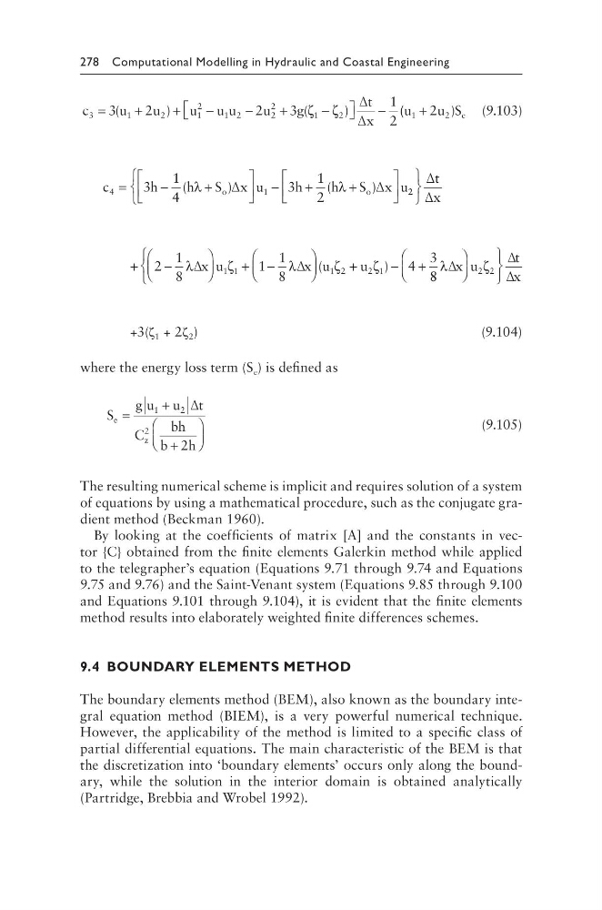
where the energy loss term (S e ) is defined as
S
g u u t
C
bh
b h
e =
+
+
1
2
2
2
∆
z
(9.105)
The resulting numerical scheme is implicit and requires solution of a system
of equations by using a mathematical procedure, such as the conjugate gradient method (Beckman 1960).
By looking at the coefficients of matrix [A] and the constants in vector {C} obtained from the finite elements Galerkin method while applied
to the telegrapher’s equation (Equations 9.71 through 9.74 and Equations
9.75 and 9.76) and the Saint-Venant system (Equations 9.85 through 9.100
and Equations 9.101 through 9.104), it is evident that the finite elements
method results into elaborately weighted finite differences schemes.
9.4 BOUNDARY ELEMENTS METHOD
The boundary elements method (BEM), also known as the boundary integral equation method (BIEM), is a very powerful numerical technique.
However, the applicability of the method is limited to a specific class of
partial differential equations. The main characteristic of the BEM is that
the discretization into ‘boundary elements’ occurs only along the boundary, while the solution in the interior domain is obtained analytically
(Partridge, Brebbia and Wrobel 1992).
c
u
u
u u u
u
g
t
x
3
1
2
1
2
1 2
2
2
1
2
3
2
2
3
1
2
=
+
+
−
−
+
−
−
(
)
(
)
ζ ζ
∆
∆
( (
)
u
u S e
1
2
2
+
(9.103)
c
h
h
S x u
h
h
S x u
o
o
4
1
3
1
4
3
1
2
=
−
+
−
+
+
(
)
(
)
λ
λ
∆
∆
2 2
∆
∆
t
x
+
−
+ −
+
− +
2
1
8
1
1
8
4
3
1 1
1 2
2 1
λ
ζ
λ
ζ
ζ
∆
∆
x u
x u
u
(
)
8 8
2 2
λ
ζ
∆
∆
∆
x u
t
x
+3(ζ 1 + 2ζ 2 )
(9.104)
where the energy loss term (S e ) is defined as
S
g u u t
C
bh
b h
e =
+
+
1
2
2
2
∆
z
(9.105)
The resulting numerical scheme is implicit and requires solution of a system
of equations by using a mathematical procedure, such as the conjugate gradient method (Beckman 1960).
By looking at the coefficients of matrix [A] and the constants in vector {C} obtained from the finite elements Galerkin method while applied
to the telegrapher’s equation (Equations 9.71 through 9.74 and Equations
9.75 and 9.76) and the Saint-Venant system (Equations 9.85 through 9.100
and Equations 9.101 through 9.104), it is evident that the finite elements
method results into elaborately weighted finite differences schemes.
9.4 BOUNDARY ELEMENTS METHOD
The boundary elements method (BEM), also known as the boundary integral equation method (BIEM), is a very powerful numerical technique.
However, the applicability of the method is limited to a specific class of
partial differential equations. The main characteristic of the BEM is that
the discretization into ‘boundary elements’ occurs only along the boundary, while the solution in the interior domain is obtained analytically
(Partridge, Brebbia and Wrobel 1992).