

Other numerical methods 275
where
ξ
ξξ
ξ
o
k
i
i
k
x x x
x
=
=
−
+
−
2
1
(
)
∆
(9.82)
η ηη
η
o
k
j
j
k
t t
t
t
=
=
−
+
+
2
1
(
)
∆
(9.83)
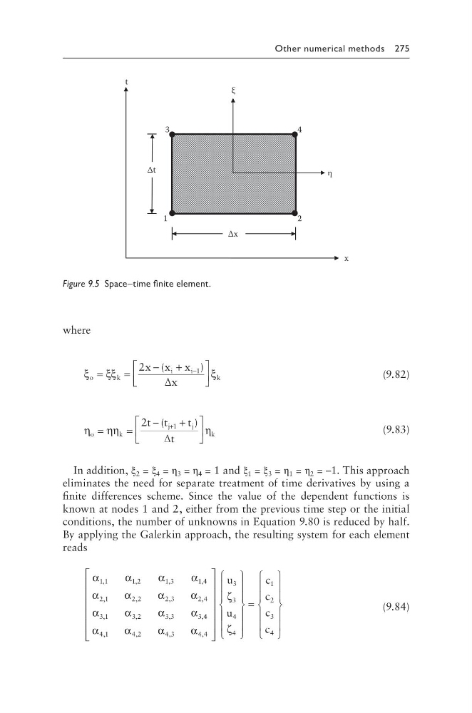
In addition, ξ 2 = ξ 4 = η 3 = η 4 = 1 and ξ 1 = ξ 3 = η 1 = η 2 = –1. This approach
eliminates the need for separate treatment of time derivatives by using a
finite differences scheme. Since the value of the dependent functions is
known at nodes 1 and 2, either from the previous time step or the initial
conditions, the number of unknowns in Equation 9.80 is reduced by half.
By applying the Galerkin approach, the resulting system for each element
reads
α
α
α
α
α
α
α
α
α
α
α
α
1 1
1 2
1 3
1 4
2 1
2 2
2 3
2 4
3 1
3 2
3 3
3
,
,
,
,
,
,
,
,
,
,
,
, 4 4
4 1
4 2
4 3
4 4
3
3
4
4
α
α
α
α
ζ
ζ
,
,
,
,
u
u
=
c
c
c
c
1
2
3
4
(9.84)
t
x
4
3
2
1
η
ξ
Δt
Δx
Figure 9.5 Space–time finite element.
where
ξ
ξξ
ξ
o
k
i
i
k
x x x
x
=
=
−
+
−
2
1
(
)
∆
(9.82)
η ηη
η
o
k
j
j
k
t t
t
t
=
=
−
+
+
2
1
(
)
∆
(9.83)
In addition, ξ 2 = ξ 4 = η 3 = η 4 = 1 and ξ 1 = ξ 3 = η 1 = η 2 = –1. This approach
eliminates the need for separate treatment of time derivatives by using a
finite differences scheme. Since the value of the dependent functions is
known at nodes 1 and 2, either from the previous time step or the initial
conditions, the number of unknowns in Equation 9.80 is reduced by half.
By applying the Galerkin approach, the resulting system for each element
reads
α
α
α
α
α
α
α
α
α
α
α
α
1 1
1 2
1 3
1 4
2 1
2 2
2 3
2 4
3 1
3 2
3 3
3
,
,
,
,
,
,
,
,
,
,
,
, 4 4
4 1
4 2
4 3
4 4
3
3
4
4
α
α
α
α
ζ
ζ
,
,
,
,
u
u
=
c
c
c
c
1
2
3
4
(9.84)
t
x
4
3
2
1
η
ξ
Δt
Δx
Figure 9.5 Space–time finite element.