

14 Computational Modelling in Hydraulic and Coastal Engineering
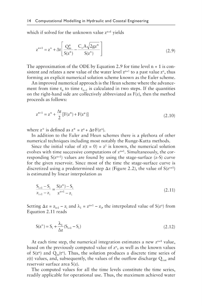
which if solved for the unknown value z n+1 yields
z
z
t
Q
S z
C A gz
S z
n
n
in
n
n
o
n
n
+
= +
−
1
2
∆ ( )
( )
(2.9)
The approximation of the ODE by Equation 2.9 for time level n + 1 is consistent and relates a new value of the water level z n+1 to a past value z n , thus
forming an explicit numerical solution scheme known as the Euler scheme.
An improved numerical approach is the Heun scheme where the advancement from time t n to time t n+1 is calculated in two steps. If the quantities
on the right-hand side are collectively abbreviated as F(z), then the method
proceeds as follows:
z
z
t F z
F z
n
n
n
+
= +
+
1
2
∆ [ ( ) ( *)]
(2.10)
where z* is defined as z* = z n + Δt·F(z n ).
In addition to the Euler and Heun schemes there is a plethora of other
numerical techniques including most notably the Runge-Kutta methods.
Since the initial value of z(t = 0) = z 1 is known, the numerical solution
evolves with time successive computations of z n+1 . Simultaneously, the corresponding S(z n+1 ) values are found by using the stage-surface (z-S) curve
for the given reservoir. Since most of the time the stage-surface curve is
discretized using a predetermined step Δz (Figure 2.2), the value of S(z n+1 )
is estimated by linear interpolation as
S
S
z
z
S z
S
z
z
i
i
i
i
n
i
n
i
+
+
+
−
−
=
−
−
1
1
1
( )
(2.11)
Setting Δz = z i+1 – z i and λ 1 = z n+1 – z i , the interpolated value of S(z n ) from
Equation 2.11 reads
S z
S
z
S
S
n
i
i
i
( )
(
)
= +
−
+
λ 1
1
∆
(2.12)
At each time step, the numerical integration estimates a new z n+1 value,
based on the previously computed value of z n , as well as the known values
of S(z n ) and Q in (t n ). Thus, the solution produces a discrete time series of
z(t) values, and, subsequently, the values of the outflow discharge Q out and
reservoir surface area S(z).
The computed values for all the time levels constitute the time series,
readily applicable for operational use. Thus, the maximum achieved water
which if solved for the unknown value z n+1 yields
z
z
t
Q
S z
C A gz
S z
n
n
in
n
n
o
n
n
+
= +
−
1
2
∆ ( )
( )
(2.9)
The approximation of the ODE by Equation 2.9 for time level n + 1 is consistent and relates a new value of the water level z n+1 to a past value z n , thus
forming an explicit numerical solution scheme known as the Euler scheme.
An improved numerical approach is the Heun scheme where the advancement from time t n to time t n+1 is calculated in two steps. If the quantities
on the right-hand side are collectively abbreviated as F(z), then the method
proceeds as follows:
z
z
t F z
F z
n
n
n
+
= +
+
1
2
∆ [ ( ) ( *)]
(2.10)
where z* is defined as z* = z n + Δt·F(z n ).
In addition to the Euler and Heun schemes there is a plethora of other
numerical techniques including most notably the Runge-Kutta methods.
Since the initial value of z(t = 0) = z 1 is known, the numerical solution
evolves with time successive computations of z n+1 . Simultaneously, the corresponding S(z n+1 ) values are found by using the stage-surface (z-S) curve
for the given reservoir. Since most of the time the stage-surface curve is
discretized using a predetermined step Δz (Figure 2.2), the value of S(z n+1 )
is estimated by linear interpolation as
S
S
z
z
S z
S
z
z
i
i
i
i
n
i
n
i
+
+
+
−
−
=
−
−
1
1
1
( )
(2.11)
Setting Δz = z i+1 – z i and λ 1 = z n+1 – z i , the interpolated value of S(z n ) from
Equation 2.11 reads
S z
S
z
S
S
n
i
i
i
( )
(
)
= +
−
+
λ 1
1
∆
(2.12)
At each time step, the numerical integration estimates a new z n+1 value,
based on the previously computed value of z n , as well as the known values
of S(z n ) and Q in (t n ). Thus, the solution produces a discrete time series of
z(t) values, and, subsequently, the values of the outflow discharge Q out and
reservoir surface area S(z).
The computed values for all the time levels constitute the time series,
readily applicable for operational use. Thus, the maximum achieved water