

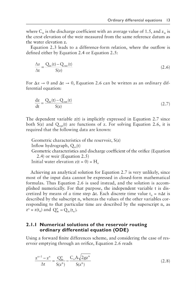
Ordinary differential equations 13
where C w is the discharge coefficient with an average value of 1.5, and z w is
the crest elevation of the weir measured from the same reference datum as
the water elevation z.
Equation 2.3 leads to a difference-form relation, where the outflow is
defined either by Equation 2.4 or Equation 2.5:
∆
∆
z
t
Q t Q t
S z
in
out
=
−
( )
( )
( )
(2.6)
For Δz → 0 and Δt → 0, Equation 2.6 can be written as an ordinary differential equation:
dz
dt
Q t Q t
S z
in
out
=
−
( )
( )
( )
(2.7)
The dependent variable z(t) is implicitly expressed in Equation 2.7 since
both S(z) and Q out (t) are functions of z. For solving Equation 2.6, it is
required that the following data are known:
Geometric characteristics of the reservoir, S(z)
Inflow hydrograph, Q in (t)
Geometric characteristics and discharge coefficient of the orifice (Equation
2.4) or weir (Equation 2.5)
Initial water elevation z(t = 0) = H o
Achieving an analytical solution for Equation 2.7 is very unlikely, since
most of the input data cannot be expressed in closed-form mathematical
formulas. Thus Equation 2.6 is used instead, and the solution is accomplished numerically. For that purpose, the independent variable t is discretized by means of a time step Δt. Each discrete time value t n = nΔt is
described by the subscript n, whereas the values of the other variables corresponding to that particular time are described by the superscript n, as
z n = z(t n ) and Q
Q t
in
n
in n
=
( ).
2.1.1 Numerical solutions of the reservoir routing
ordinary differential equation (ODE)
Using a forward finite differences scheme, and considering the case of reservoir emptying through an orifice, Equation 2.6 reads
z
z
t
Q
S z
C A gz
S z
n
n
in
n
n
o
n
n
+
− =
−
1
2
∆
( )
( )
(2.8)
where C w is the discharge coefficient with an average value of 1.5, and z w is
the crest elevation of the weir measured from the same reference datum as
the water elevation z.
Equation 2.3 leads to a difference-form relation, where the outflow is
defined either by Equation 2.4 or Equation 2.5:
∆
∆
z
t
Q t Q t
S z
in
out
=
−
( )
( )
( )
(2.6)
For Δz → 0 and Δt → 0, Equation 2.6 can be written as an ordinary differential equation:
dz
dt
Q t Q t
S z
in
out
=
−
( )
( )
( )
(2.7)
The dependent variable z(t) is implicitly expressed in Equation 2.7 since
both S(z) and Q out (t) are functions of z. For solving Equation 2.6, it is
required that the following data are known:
Geometric characteristics of the reservoir, S(z)
Inflow hydrograph, Q in (t)
Geometric characteristics and discharge coefficient of the orifice (Equation
2.4) or weir (Equation 2.5)
Initial water elevation z(t = 0) = H o
Achieving an analytical solution for Equation 2.7 is very unlikely, since
most of the input data cannot be expressed in closed-form mathematical
formulas. Thus Equation 2.6 is used instead, and the solution is accomplished numerically. For that purpose, the independent variable t is discretized by means of a time step Δt. Each discrete time value t n = nΔt is
described by the subscript n, whereas the values of the other variables corresponding to that particular time are described by the superscript n, as
z n = z(t n ) and Q
Q t
in
n
in n
=
( ).
2.1.1 Numerical solutions of the reservoir routing
ordinary differential equation (ODE)
Using a forward finite differences scheme, and considering the case of reservoir emptying through an orifice, Equation 2.6 reads
z
z
t
Q
S z
C A gz
S z
n
n
in
n
n
o
n
n
+
− =
−
1
2
∆
( )
( )
(2.8)