

6 Computational Modelling in Hydraulic and Coastal Engineering
where Δx is a small quantity. From Equation 1.2, the following equalities
can be derived:
df
dx
f x
x f x
x
O x
=
+
−
+
(
) ( )
( )
∆
∆
∆
(1.3)
df
dx
f x f x
x
x
O x
=
−
−
+
( ) (
)
( )
∆
∆
∆
(1.4)
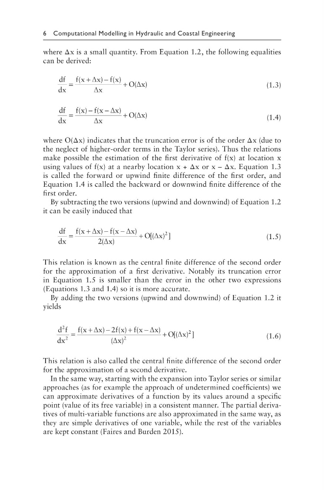
where O(Δx) indicates that the truncation error is of the order Δx (due to
the neglect of higher-order terms in the Taylor series). Thus the relations
make possible the estimation of the first derivative of f(x) at location x
using values of f(x) at a nearby location x + Δx or x – Δx. Equation 1.3
is called the forward or upwind finite difference of the first order, and
Equation 1.4 is called the backward or downwind finite difference of the
first order.
By subtracting the two versions (upwind and downwind) of Equation 1.2
it can be easily induced that
df
dx
f x
x f x
x
x
O x
=
+
−
−
+
(
) (
)
( )
[( ) ]
∆
∆
∆
∆
2
2
(1.5)
This relation is known as the central finite difference of the second order
for the approximation of a first derivative. Notably its truncation error
in Equation 1.5 is smaller than the error in the other two expressions
(Equations 1.3 and 1.4) so it is more accurate.
By adding the two versions (upwind and downwind) of Equation 1.2 it
yields
d f
dx
x
x
f x f x
x
x
O x
2
2
2
2
2
=
+
−
+
−
+
f
∆
∆
∆
∆
(
)
( ) (
)
( )
[( ) ]
(1.6)
This relation is also called the central finite difference of the second order
for the approximation of a second derivative.
In the same way, starting with the expansion into Taylor series or similar
approaches (as for example the approach of undetermined coefficients) we
can approximate derivatives of a function by its values around a specific
point (value of its free variable) in a consistent manner. The partial derivatives of multi-variable functions are also approximated in the same way, as
they are simple derivatives of one variable, while the rest of the variables
are kept constant (Faires and Burden 2015).
where Δx is a small quantity. From Equation 1.2, the following equalities
can be derived:
df
dx
f x
x f x
x
O x
=
+
−
+
(
) ( )
( )
∆
∆
∆
(1.3)
df
dx
f x f x
x
x
O x
=
−
−
+
( ) (
)
( )
∆
∆
∆
(1.4)
where O(Δx) indicates that the truncation error is of the order Δx (due to
the neglect of higher-order terms in the Taylor series). Thus the relations
make possible the estimation of the first derivative of f(x) at location x
using values of f(x) at a nearby location x + Δx or x – Δx. Equation 1.3
is called the forward or upwind finite difference of the first order, and
Equation 1.4 is called the backward or downwind finite difference of the
first order.
By subtracting the two versions (upwind and downwind) of Equation 1.2
it can be easily induced that
df
dx
f x
x f x
x
x
O x
=
+
−
−
+
(
) (
)
( )
[( ) ]
∆
∆
∆
∆
2
2
(1.5)
This relation is known as the central finite difference of the second order
for the approximation of a first derivative. Notably its truncation error
in Equation 1.5 is smaller than the error in the other two expressions
(Equations 1.3 and 1.4) so it is more accurate.
By adding the two versions (upwind and downwind) of Equation 1.2 it
yields
d f
dx
x
x
f x f x
x
x
O x
2
2
2
2
2
=
+
−
+
−
+
f
∆
∆
∆
∆
(
)
( ) (
)
( )
[( ) ]
(1.6)
This relation is also called the central finite difference of the second order
for the approximation of a second derivative.
In the same way, starting with the expansion into Taylor series or similar
approaches (as for example the approach of undetermined coefficients) we
can approximate derivatives of a function by its values around a specific
point (value of its free variable) in a consistent manner. The partial derivatives of multi-variable functions are also approximated in the same way, as
they are simple derivatives of one variable, while the rest of the variables
are kept constant (Faires and Burden 2015).