

Free surface flows 125
KinE(k)=ke;
index=k
end
[X,Y]=meshgrid(1:1:nx,1:1:ny);
[m n]=size(Y);
for a=1:m
for b=1:n
Z(a,b)=-fm(b,a,df);
end
end
surf(X,Y,Z)
figure
plot(1:k,KinE,'Color','k','Linewidth',1.5);
xlabel('Number of time steps')
ylabel('Total kinetic energy (u^2+v^2 on all grid points)')
[i,j]=meshgrid(1:1:nx,1:1:ny);
df1=df(:,3);
df2=reshape(df1,22,23);
df2=df2’;
An=ones(size(df2));
idx=find(df2==0);
An(idx)=0;
figure,pcolor(An); hold on;
colormap(bone)
shading flat
LL=quiver(i,j,u',v','Color','k');
% set(LL,'linewidth',1.5);
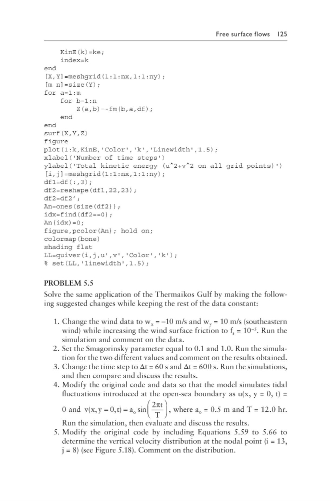
PROBLEM 5.5
Solve the same application of the Thermaikos Gulf by making the following suggested changes while keeping the rest of the data constant:
1. Change the wind data to w x = –10 m/s and w y = 10 m/s (southeastern
wind) while increasing the wind surface friction to f s = 10 –5 . Run the
simulation and comment on the data.
2. Set the Smagorinsky parameter equal to 0.1 and 1.0. Run the simulation for the two different values and comment on the results obtained.
3. Change the time step to Δt = 60 s and Δt = 600 s. Run the simulations,
and then compare and discuss the results.
4. Modify the original code and data so that the model simulates tidal
fluctuations introduced at the open-sea boundary as u(x, y = 0, t) =
0 and v x y
t a
t
T
o
( ,
, )
sin
=
=
0
2π , where a o = 0.5 m and T = 12.0 hr.
Run the simulation, then evaluate and discuss the results.
5. Modify the original code by including Equations 5.59 to 5.66 to
determine the vertical velocity distribution at the nodal point (i = 13,
j = 8) (see Figure 5.18). Comment on the distribution.
KinE(k)=ke;
index=k
end
[X,Y]=meshgrid(1:1:nx,1:1:ny);
[m n]=size(Y);
for a=1:m
for b=1:n
Z(a,b)=-fm(b,a,df);
end
end
surf(X,Y,Z)
figure
plot(1:k,KinE,'Color','k','Linewidth',1.5);
xlabel('Number of time steps')
ylabel('Total kinetic energy (u^2+v^2 on all grid points)')
[i,j]=meshgrid(1:1:nx,1:1:ny);
df1=df(:,3);
df2=reshape(df1,22,23);
df2=df2’;
An=ones(size(df2));
idx=find(df2==0);
An(idx)=0;
figure,pcolor(An); hold on;
colormap(bone)
shading flat
LL=quiver(i,j,u',v','Color','k');
% set(LL,'linewidth',1.5);
PROBLEM 5.5
Solve the same application of the Thermaikos Gulf by making the following suggested changes while keeping the rest of the data constant:
1. Change the wind data to w x = –10 m/s and w y = 10 m/s (southeastern
wind) while increasing the wind surface friction to f s = 10 –5 . Run the
simulation and comment on the data.
2. Set the Smagorinsky parameter equal to 0.1 and 1.0. Run the simulation for the two different values and comment on the results obtained.
3. Change the time step to Δt = 60 s and Δt = 600 s. Run the simulations,
and then compare and discuss the results.
4. Modify the original code and data so that the model simulates tidal
fluctuations introduced at the open-sea boundary as u(x, y = 0, t) =
0 and v x y
t a
t
T
o
( ,
, )
sin
=
=
0
2π , where a o = 0.5 m and T = 12.0 hr.
Run the simulation, then evaluate and discuss the results.
5. Modify the original code by including Equations 5.59 to 5.66 to
determine the vertical velocity distribution at the nodal point (i = 13,
j = 8) (see Figure 5.18). Comment on the distribution.