

Free surface flows 107
The non-linear terms of the total (material) derivatives Du/Dt and Dv/Dt
tend to produce numerical instabilities and chaotic solutions. The frictional
terms tend to stabilize the flow and the diffusive terms tend to smooth the
functional forms and diminish the development of numerical instabilities.
Notably, the equations contain both hyperbolic and parabolic terms.
The selection of the spatial-temporal distribution and magnitude of the
horizontal eddy viscosity coefficient, ε h , is a concurrent problem of the ‘turbulence closure’. That coefficient can be used as a controller of the numerical stability and its influence can be merged with the numerical diffusion
error. The coefficient ε h can be properly adjusted either to permit the
description of eddies of certain geometric and energy scale, or to diffuse
them letting only more basic features of the flow appear in the solution.
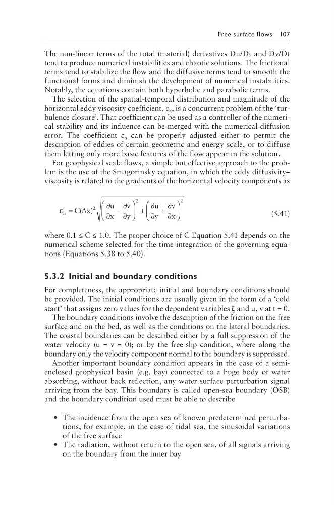
For geophysical scale flows, a simple but effective approach to the problem is the use of the Smagorinsky equation, in which the eddy diffusivity–
viscosity is related to the gradients of the horizontal velocity components as
ε h C x
u
x
v
y
u
y
v
x
=
∂
∂
−
∂
∂
+
∂
∂
+
∂
∂
( )
∆
2
2
2
(5.41)
where 0.1 ≤ C ≤ 1.0. The proper choice of C Equation 5.41 depends on the
numerical scheme selected for the time-integration of the governing equations (Equations 5.38 to 5.40).
5.3.2 Initial and boundary conditions
For completeness, the appropriate initial and boundary conditions should
be provided. The initial conditions are usually given in the form of a ‘cold
start’ that assigns zero values for the dependent variables ζ and u, v at t = 0.
The boundary conditions involve the description of the friction on the free
surface and on the bed, as well as the conditions on the lateral bound aries.
The coastal boundaries can be described either by a full suppression of the
water velocity (u = v = 0); or by the free-slip condition, where along the
boundary only the velocity component normal to the boundary is suppressed.
Another important boundary condition appears in the case of a semienclosed geophysical basin (e.g. bay) connected to a huge body of water
absorbing, without back reflection, any water surface perturbation signal
arriving from the bay. This boundary is called open-sea boundary (OSB)
and the boundary condition used must be able to describe
• The incidence from the open sea of known predetermined perturbations, for example, in the case of tidal sea, the sinusoidal variations
of the free surface
• The radiation, without return to the open sea, of all signals arriving
on the boundary from the inner bay
The non-linear terms of the total (material) derivatives Du/Dt and Dv/Dt
tend to produce numerical instabilities and chaotic solutions. The frictional
terms tend to stabilize the flow and the diffusive terms tend to smooth the
functional forms and diminish the development of numerical instabilities.
Notably, the equations contain both hyperbolic and parabolic terms.
The selection of the spatial-temporal distribution and magnitude of the
horizontal eddy viscosity coefficient, ε h , is a concurrent problem of the ‘turbulence closure’. That coefficient can be used as a controller of the numerical stability and its influence can be merged with the numerical diffusion
error. The coefficient ε h can be properly adjusted either to permit the
description of eddies of certain geometric and energy scale, or to diffuse
them letting only more basic features of the flow appear in the solution.
For geophysical scale flows, a simple but effective approach to the problem is the use of the Smagorinsky equation, in which the eddy diffusivity–
viscosity is related to the gradients of the horizontal velocity components as
ε h C x
u
x
v
y
u
y
v
x
=
∂
∂
−
∂
∂
+
∂
∂
+
∂
∂
( )
∆
2
2
2
(5.41)
where 0.1 ≤ C ≤ 1.0. The proper choice of C Equation 5.41 depends on the
numerical scheme selected for the time-integration of the governing equations (Equations 5.38 to 5.40).
5.3.2 Initial and boundary conditions
For completeness, the appropriate initial and boundary conditions should
be provided. The initial conditions are usually given in the form of a ‘cold
start’ that assigns zero values for the dependent variables ζ and u, v at t = 0.
The boundary conditions involve the description of the friction on the free
surface and on the bed, as well as the conditions on the lateral bound aries.
The coastal boundaries can be described either by a full suppression of the
water velocity (u = v = 0); or by the free-slip condition, where along the
boundary only the velocity component normal to the boundary is suppressed.
Another important boundary condition appears in the case of a semienclosed geophysical basin (e.g. bay) connected to a huge body of water
absorbing, without back reflection, any water surface perturbation signal
arriving from the bay. This boundary is called open-sea boundary (OSB)
and the boundary condition used must be able to describe
• The incidence from the open sea of known predetermined perturbations, for example, in the case of tidal sea, the sinusoidal variations
of the free surface
• The radiation, without return to the open sea, of all signals arriving
on the boundary from the inner bay