

Free surface flows 99
3. Change the inflow hydrograph to Q = 0 m 3 /s at t = 0 s; Q = 1000 m 3 /s
at t = 2000 s; Q = 0 m 3 /s at t = 4000 s; Q = 1000 m 3 /s at t = 6000 s;
and Q = 0 m 3 /s at t = 8000 s. Assume a linear variation of the hydrographs between the time intervals δt = 2000 s. Run the program and
comment on the results.
4. By using the appropriate expression, change the downstream boundary to a zero-flux (reflecting) boundary. Comment on the results.
5. Change the computational time step to Δt = 400 s. Comment on the
results.
Example 5.3
This exercise investigates the routing of a sudden-release (dam-break)
flood wave in a natural stream of variable width. The data used for the
simulation are as follows:
Channel length = 46,000 m
Bed slope = 0.0004
Chezy’s coefficient of friction = 40 m 1/2 /s
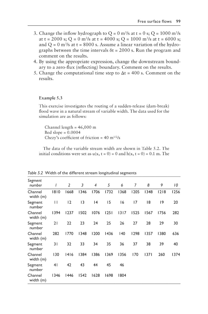
The data of the variable stream width are shown in Table 5.2. The
initial conditions were set as u(x, t = 0) = 0 and h(x, t = 0) = 0.1 m. The
Table 5.2 Width of the different stream longitudinal segments
Segment
number
1
2
3
4
5
6
7
8
9
10
Channel
width (m)
1810 1668 1346 1706 1732 1368 1205 1348 1218 1256
Segment
number
11
12
13
14
15
16
17
18
19
20
Channel
width (m)
1394 1237 1502 1076 1251 1317 1525 1567 1756
282
Segment
number
21
22
23
24
25
26
27
28
29
30
Channel
width (m)
282 1770 1348 1200 1436 140 1298 1357 1380
636
Segment
number
31
32
33
34
35
36
37
38
39
40
Channel
width (m)
130 1416 1384 1386 1369 1356 170 1371 260
1374
Segment
number
41
42
43
44
45
46
Channel
width (m)
1346 1446 1542 1628 1698 1804
3. Change the inflow hydrograph to Q = 0 m 3 /s at t = 0 s; Q = 1000 m 3 /s
at t = 2000 s; Q = 0 m 3 /s at t = 4000 s; Q = 1000 m 3 /s at t = 6000 s;
and Q = 0 m 3 /s at t = 8000 s. Assume a linear variation of the hydrographs between the time intervals δt = 2000 s. Run the program and
comment on the results.
4. By using the appropriate expression, change the downstream boundary to a zero-flux (reflecting) boundary. Comment on the results.
5. Change the computational time step to Δt = 400 s. Comment on the
results.
Example 5.3
This exercise investigates the routing of a sudden-release (dam-break)
flood wave in a natural stream of variable width. The data used for the
simulation are as follows:
Channel length = 46,000 m
Bed slope = 0.0004
Chezy’s coefficient of friction = 40 m 1/2 /s
The data of the variable stream width are shown in Table 5.2. The
initial conditions were set as u(x, t = 0) = 0 and h(x, t = 0) = 0.1 m. The
Table 5.2 Width of the different stream longitudinal segments
Segment
number
1
2
3
4
5
6
7
8
9
10
Channel
width (m)
1810 1668 1346 1706 1732 1368 1205 1348 1218 1256
Segment
number
11
12
13
14
15
16
17
18
19
20
Channel
width (m)
1394 1237 1502 1076 1251 1317 1525 1567 1756
282
Segment
number
21
22
23
24
25
26
27
28
29
30
Channel
width (m)
282 1770 1348 1200 1436 140 1298 1357 1380
636
Segment
number
31
32
33
34
35
36
37
38
39
40
Channel
width (m)
130 1416 1384 1386 1369 1356 170 1371 260
1374
Segment
number
41
42
43
44
45
46
Channel
width (m)
1346 1446 1542 1628 1698 1804