

42
STRUCTURE-ENVIRONMENTAL FORCE INTERACTIONS
forces on m are shown on the free body sketch in Figure 2.16e, from which the
équation of motion is deduced as
mv + Civ + k^v = pi(t)
(2.43)
Here, since pi (t) is ail lumped at midspan instead of being uniformly distributed,
the solution v = v(t) to équation (2.43) will be on the high side. This particular
mathematical model is thus a conservative one. Needed for py (t) are the explicit
forms for the flow field u = u(t) and its associated constants CD and CM, topics
that are deferred to Chapters 3 and 4.
(a) TYPICAL STRUCTURE
(b) MATHEMATICAL
(DIMENSIONS: ft)
MODEL
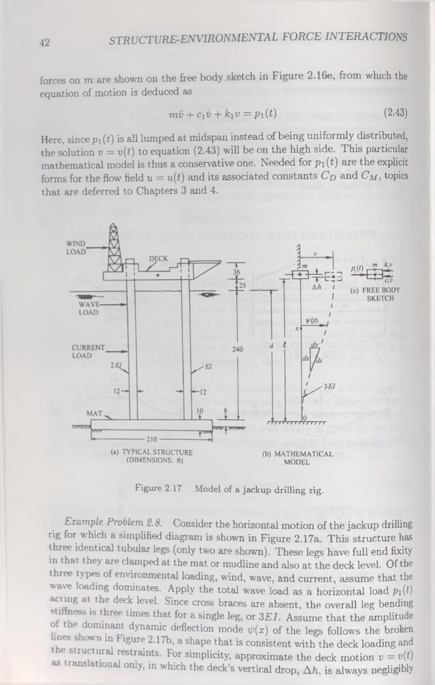
Figure 2.17 Model of a jackup drilling rig.
Erample Problem 2.8. Consider the horizontal motion of the jackup drilling
rig for which a simplified diagram is shown in Figure 2.17a. This structure has
three identical tubular legs (only two are shown). These legs hâve full end fixity
in that they are clamped at the mat or mudline and also at the deck level. Of the
three tjpes of environmental loading, wind, wave, and current, assume that the
wave loading dominâtes. Apply the total wave load as a horizontal load pi(i)
acting at the deck level. Since cross braces are absent, the overall leg bending
sti ness is t hree times that for a single leg, or 3EI. Assume that the amplitude
ot the dominant dynamic deflection mode ^(x) of the legs follows the broken
nés s wn in Figure 2.17b, a shape that is consistent with the deck loading and
the structural restraints. For simplicity, approximate the deck motion v = v(i)
as translatai only, in which the deck’s vertical drop, Ah, is always negligibly
STRUCTURE-ENVIRONMENTAL FORCE INTERACTIONS
forces on m are shown on the free body sketch in Figure 2.16e, from which the
équation of motion is deduced as
mv + Civ + k^v = pi(t)
(2.43)
Here, since pi (t) is ail lumped at midspan instead of being uniformly distributed,
the solution v = v(t) to équation (2.43) will be on the high side. This particular
mathematical model is thus a conservative one. Needed for py (t) are the explicit
forms for the flow field u = u(t) and its associated constants CD and CM, topics
that are deferred to Chapters 3 and 4.
(a) TYPICAL STRUCTURE
(b) MATHEMATICAL
(DIMENSIONS: ft)
MODEL
Figure 2.17 Model of a jackup drilling rig.
Erample Problem 2.8. Consider the horizontal motion of the jackup drilling
rig for which a simplified diagram is shown in Figure 2.17a. This structure has
three identical tubular legs (only two are shown). These legs hâve full end fixity
in that they are clamped at the mat or mudline and also at the deck level. Of the
three tjpes of environmental loading, wind, wave, and current, assume that the
wave loading dominâtes. Apply the total wave load as a horizontal load pi(i)
acting at the deck level. Since cross braces are absent, the overall leg bending
sti ness is t hree times that for a single leg, or 3EI. Assume that the amplitude
ot the dominant dynamic deflection mode ^(x) of the legs follows the broken
nés s wn in Figure 2.17b, a shape that is consistent with the deck loading and
the structural restraints. For simplicity, approximate the deck motion v = v(i)
as translatai only, in which the deck’s vertical drop, Ah, is always negligibly