

EARTHQUAKES, ICE IMPACT, AND WAVE SLAMMING
37
A typical earthquake-induced ground accélération time history, which is
sometimes used as input to the base of a structure to evaluate its earthquake
résistance, is shown in Figure 2.14. Here the horizontal ground accélération vg
is expressed as a multiple of g, the accélération due to gravity. The instantaneous upper bound on this accélération is approximateiy 0.3$. For the largest
California earthquakes on firm, deep alluvium, the total time for destructive
shaking is about 45 seconds. The following example illustrâtes how such data
can be used as a driving force for a simple model of an offshore structure.
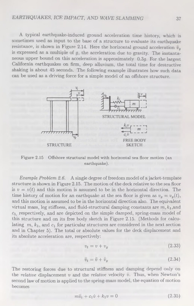
Figure 2.15 Offshore structural model with horizontal sea floor motion (an
earthquake).
Example Problem 2.6. A single degree of freedom model of a jacket-template
structure is shown in Figure 2.15. The motion of the deck relative to the sea floor
is v = v(é) and this motion is assumed to be in the horizontal direction. The
time history of motion for an earthquake at the sea floor is given as vg — vg(t),
and this motion is assumed to be in the horizontal direction also. The équivalent
virtual mass, leg stiffness, and fluid-structural damping constants are m, Aq,and
Ci, respectively, and are depicted on the simple damped, spring-mass model of
this structure and on its free body sketch in Figure 2.15. (Methods for calculating m, ki, and Ci for particular structures are considered in the next section
and in Chapter 5). The total or absolute values for the deck displacement and
its absolute accélération are, respectively:
vt = v + vg
(2.33)
vt = v + vg
(2.34)
The restoring forces due to structural stiffness and damping dépend only on
the relative displacement v and the relative velocity v. Thus, when Newton’s
second law of motion is applied to the spring-mass model, the équation of motion
becomes
mvt + cjû 4- k\v = 0
(2.35)
37
A typical earthquake-induced ground accélération time history, which is
sometimes used as input to the base of a structure to evaluate its earthquake
résistance, is shown in Figure 2.14. Here the horizontal ground accélération vg
is expressed as a multiple of g, the accélération due to gravity. The instantaneous upper bound on this accélération is approximateiy 0.3$. For the largest
California earthquakes on firm, deep alluvium, the total time for destructive
shaking is about 45 seconds. The following example illustrâtes how such data
can be used as a driving force for a simple model of an offshore structure.
Figure 2.15 Offshore structural model with horizontal sea floor motion (an
earthquake).
Example Problem 2.6. A single degree of freedom model of a jacket-template
structure is shown in Figure 2.15. The motion of the deck relative to the sea floor
is v = v(é) and this motion is assumed to be in the horizontal direction. The
time history of motion for an earthquake at the sea floor is given as vg — vg(t),
and this motion is assumed to be in the horizontal direction also. The équivalent
virtual mass, leg stiffness, and fluid-structural damping constants are m, Aq,and
Ci, respectively, and are depicted on the simple damped, spring-mass model of
this structure and on its free body sketch in Figure 2.15. (Methods for calculating m, ki, and Ci for particular structures are considered in the next section
and in Chapter 5). The total or absolute values for the deck displacement and
its absolute accélération are, respectively:
vt = v + vg
(2.33)
vt = v + vg
(2.34)
The restoring forces due to structural stiffness and damping dépend only on
the relative displacement v and the relative velocity v. Thus, when Newton’s
second law of motion is applied to the spring-mass model, the équation of motion
becomes
mvt + cjû 4- k\v = 0
(2.35)