

292
BEHAVIOR OF PILES SUPPORTING OFFSHORE STRUCTURES
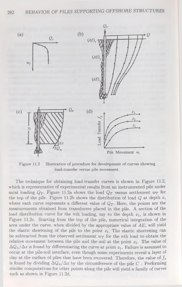
Figure 11.2 Illustration of procedure for development of curves showing
load-transfer versus pile movement.
The technique for obtaining load-transfer curves is shown in Figure 11.2,
which is représentative of experimental results from an instrumented pile under
axial loading Qp. Figure 11.2a shows the load Qp versus settlement wp for
the top of the pile. Figure 11.2b shows the distribution of load Q at depth x,
where each curve represents a different value of Qp. Here, the points are the
measurements obtained from transducers placed in the pile. A section of the
load distribution curve for the nth loading, say to the depth z15 is shown in
Figure 11.2c. Starting from the top of the pile, numerical intégration of the
area under the curve, when divided by the appropriate value of AE, will yield
the elastic shortening of the pile to the point zL The elastic shortening can
be subtracted from the observed settlement wp for the nth load to obtain the
relative movement between the pile and the soil at the point Z\. The value of
AQn/kz is found by differentiating the curve at point zx. Failure is assumed to
occur at the pile-soil interface, even though some experiments reveal a layer of
clay at the surface of piles that hâve been recovered. Therefore, the value of fz
is found by dividing &QnIAz by the circumference of the pile C . Performing
similar computations for other points along the pile will yield a family of curves
such as shown in Figure 11.2d.
BEHAVIOR OF PILES SUPPORTING OFFSHORE STRUCTURES
Figure 11.2 Illustration of procedure for development of curves showing
load-transfer versus pile movement.
The technique for obtaining load-transfer curves is shown in Figure 11.2,
which is représentative of experimental results from an instrumented pile under
axial loading Qp. Figure 11.2a shows the load Qp versus settlement wp for
the top of the pile. Figure 11.2b shows the distribution of load Q at depth x,
where each curve represents a different value of Qp. Here, the points are the
measurements obtained from transducers placed in the pile. A section of the
load distribution curve for the nth loading, say to the depth z15 is shown in
Figure 11.2c. Starting from the top of the pile, numerical intégration of the
area under the curve, when divided by the appropriate value of AE, will yield
the elastic shortening of the pile to the point zL The elastic shortening can
be subtracted from the observed settlement wp for the nth load to obtain the
relative movement between the pile and the soil at the point Z\. The value of
AQn/kz is found by differentiating the curve at point zx. Failure is assumed to
occur at the pile-soil interface, even though some experiments reveal a layer of
clay at the surface of piles that hâve been recovered. Therefore, the value of fz
is found by dividing &QnIAz by the circumference of the pile C . Performing
similar computations for other points along the pile will yield a family of curves
such as shown in Figure 11.2d.