

274
CONTINUOUS SYSTEMS
resulting équation by Xm = Xm(x), and integrate each term over the interval
(0,£). Applying the orthogonality conditions (10.70) and (10.71), the resuit is
1 Ie
=
Xnq(x,t)dx
(10.116)
^0 Jo
Co= / X2dx
(10.117)
Jo
With équation (10.115), this generalized load becomes
=
l‘Xn \G(w)\dx
(10.118)
b-o JO
Note that for a horizontal beam normal to simple, incident plane waves, G(w)
does not dépend on the beam’s longitudinal coordinate x. However, for a vertical
beam such as a pile subjected to these same waves, then G(w) does dépend on
the beam’s longitudinal coordinate x, and two adjustments in nomenclature for
the wave theory appearing in Chapter 3 are in order. The first adjustment is to
replace the depth coordinate z in the wave theory by z = — x. Thus, the origin
of the beam coordinate is at the still water line and is positive downward. The
second adjustment is to let x = 0 in the wave theory, which puts the origin of
the wave at the location of the vertical beam.
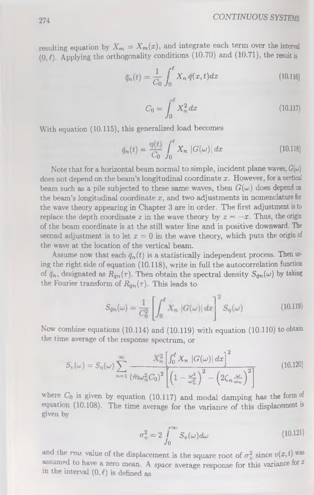
Assume now that each qn(t) is a statistically independent process. Then using the right side of équation (10.118), write in full the autocorrélation function
of qn, designated as Hqn(r). Then obtain the spectral density S^n(w) by taking
the Fourier transform of 77Qn(r). This leads to
Now combine équations (10.114) and (10.119) with équation (10.110) to obtain
the time average of the response spectrum, or
S1.u) = s„(ta,)^----------"=* (rnw2Cof
(10.120)
where Cq is given by équation (10.117) and modal damping has the form of
équation (10.108). The time average for the variance of this displacement is
given by
roo
and t he nm value of the displacement is the square root of n'2 since v(x, t) was
assumed to hâve a zéro mean. A space average response for this variance for I
in the interval (0, €) is defined as
CONTINUOUS SYSTEMS
resulting équation by Xm = Xm(x), and integrate each term over the interval
(0,£). Applying the orthogonality conditions (10.70) and (10.71), the resuit is
1 Ie
=
Xnq(x,t)dx
(10.116)
^0 Jo
Co= / X2dx
(10.117)
Jo
With équation (10.115), this generalized load becomes
=
l‘Xn \G(w)\dx
(10.118)
b-o JO
Note that for a horizontal beam normal to simple, incident plane waves, G(w)
does not dépend on the beam’s longitudinal coordinate x. However, for a vertical
beam such as a pile subjected to these same waves, then G(w) does dépend on
the beam’s longitudinal coordinate x, and two adjustments in nomenclature for
the wave theory appearing in Chapter 3 are in order. The first adjustment is to
replace the depth coordinate z in the wave theory by z = — x. Thus, the origin
of the beam coordinate is at the still water line and is positive downward. The
second adjustment is to let x = 0 in the wave theory, which puts the origin of
the wave at the location of the vertical beam.
Assume now that each qn(t) is a statistically independent process. Then using the right side of équation (10.118), write in full the autocorrélation function
of qn, designated as Hqn(r). Then obtain the spectral density S^n(w) by taking
the Fourier transform of 77Qn(r). This leads to
Now combine équations (10.114) and (10.119) with équation (10.110) to obtain
the time average of the response spectrum, or
S1.u) = s„(ta,)^----------"=* (rnw2Cof
(10.120)
where Cq is given by équation (10.117) and modal damping has the form of
équation (10.108). The time average for the variance of this displacement is
given by
roo
and t he nm value of the displacement is the square root of n'2 since v(x, t) was
assumed to hâve a zéro mean. A space average response for this variance for I
in the interval (0, €) is defined as