

beam responses
271
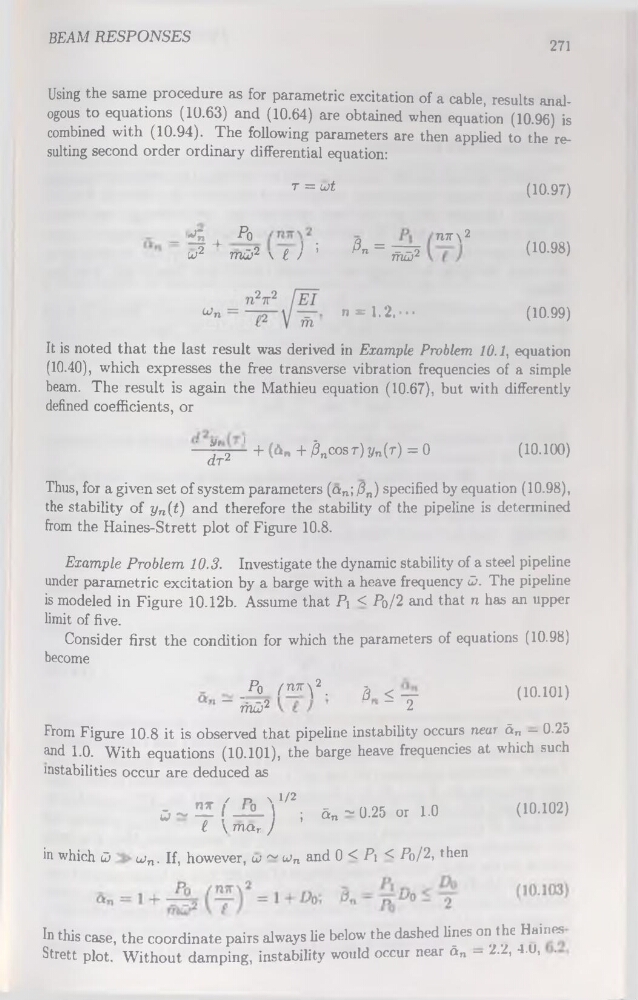
Using the same procedure as for parametric excitation of a cable, results analogous to équations (10.63) and (10.64) are obtained when équation (10.96) is
combined with (10.94). The following parameters are then applied to the resulting second order ordinary differential équation:
T = U)t
(10.97)
iS 4- P°
.
w2
mû2 \ t ) ’
0 = ~
t-'n
--- o
mor
nir\2
(10.98)
n = 1.2, ...
(10.99)
It is noted that the last resuit was derived in Example Problem 10.1, équation
(10.40), which expresses the free transverse vibration frequencies of a simple
beam. The resuit is again the Mathieu équation (10.67), but with differently
defined coefficients, or
' ^_2 ' + (Û» + 3nCOST) l/n(f) = 0
(10.100)
Thus, for a given set of System parameters (ûn; 0n) specified by équation (10.98),
the stability of j/n(t) and therefore the stability of the pipeline is detennined
from the Haines-Strett plot of Figure 10.8.
Example Problem 10.3. Investigate the dynamic stability of a Steel pipeline
under parametric excitation by a barge with a heave frequency û>. The pipeline
is modeled in Figure 10.12b. Assume that Pi < Po/2 and that n has an upper
lirait of five.
Consider first the condition for which the parameters of équations (10.98)
become
P° £n7rVâ< —
- /W
S 2
(10.101)
From Figure 10.8 it is observed that pipeline instability occurs near ân — 0.25
and 1.0. With équations (10.101), the barge heave frequencies at which such
rastabilities occur are deduced as
, n x t/2
□ ~ 21 I 2L )
; ân - 0.25 or 1.0
(10.102)
£ \marJ
in which ü
u>n. If, however, w ~ wn and 0 < Pi < Po/2, then
In this case, the coordinate pairs always lie below the dashed Unes on the Haines
Strett plot. Without damping, instabihty would occur near ân — 2.2, 4.U, .
271
Using the same procedure as for parametric excitation of a cable, results analogous to équations (10.63) and (10.64) are obtained when équation (10.96) is
combined with (10.94). The following parameters are then applied to the resulting second order ordinary differential équation:
T = U)t
(10.97)
iS 4- P°
.
w2
mû2 \ t ) ’
0 = ~
t-'n
--- o
mor
nir\2
(10.98)
n = 1.2, ...
(10.99)
It is noted that the last resuit was derived in Example Problem 10.1, équation
(10.40), which expresses the free transverse vibration frequencies of a simple
beam. The resuit is again the Mathieu équation (10.67), but with differently
defined coefficients, or
' ^_2 ' + (Û» + 3nCOST) l/n(f) = 0
(10.100)
Thus, for a given set of System parameters (ûn; 0n) specified by équation (10.98),
the stability of j/n(t) and therefore the stability of the pipeline is detennined
from the Haines-Strett plot of Figure 10.8.
Example Problem 10.3. Investigate the dynamic stability of a Steel pipeline
under parametric excitation by a barge with a heave frequency û>. The pipeline
is modeled in Figure 10.12b. Assume that Pi < Po/2 and that n has an upper
lirait of five.
Consider first the condition for which the parameters of équations (10.98)
become
P° £n7rVâ< —
- /W
S 2
(10.101)
From Figure 10.8 it is observed that pipeline instability occurs near ân — 0.25
and 1.0. With équations (10.101), the barge heave frequencies at which such
rastabilities occur are deduced as
, n x t/2
□ ~ 21 I 2L )
; ân - 0.25 or 1.0
(10.102)
£ \marJ
in which ü
u>n. If, however, w ~ wn and 0 < Pi < Po/2, then
In this case, the coordinate pairs always lie below the dashed Unes on the Haines
Strett plot. Without damping, instabihty would occur near ân — 2.2, 4.U, .