

262
CONTINUOUS SYSTEMS
The resuit is the fainous Mathieu équation, which is
d
+ (ûn + 0n cos r) yn(r) = 0
(10.67)
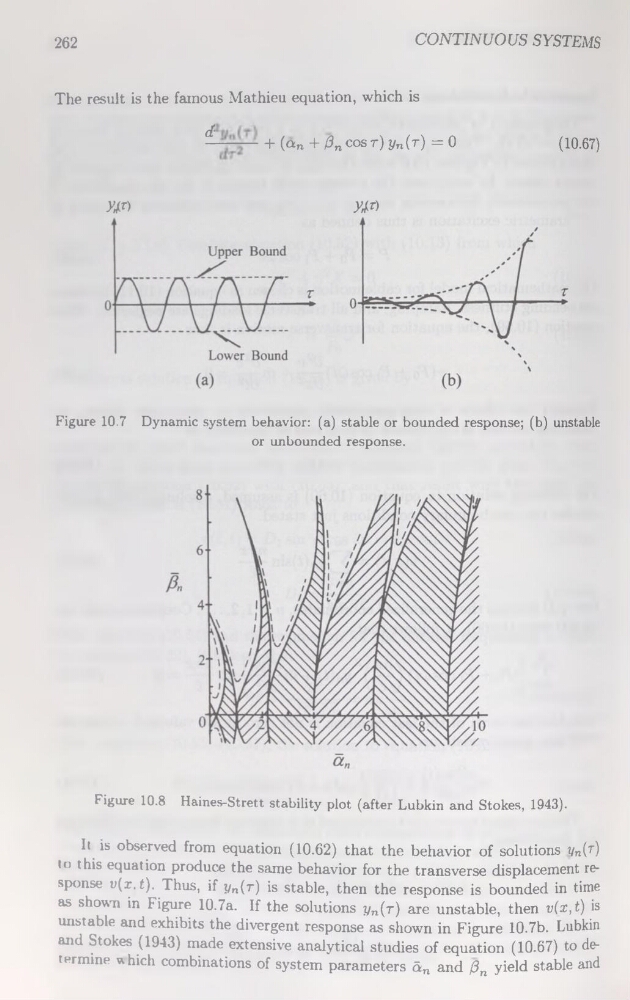
Figure 10.7 Dynamic System behavior: (a) stable or bounded response; (b) unstable
or unbounded response.
Figure 10.8 Haines-Strett stability plot (after Lubkin and Stokes, 1943).
It is observed from équation (10.62) that the behavior of solutions yn(T)
to this équation produce the same behavior for the transverse displacement response v(r.t). Thus, if yn(r) is stable, then the response is bounded in time
as shown in Figure 10.7a. If the solutions yn(r) are unstable, then v(x,t) is
unstable and exhibits the divergent response as shown in Figure 10.7b. Lubkin
and Stokes (1943) made extensive analytical studies of équation (10.67) to determine which combinations of System parameters ân and /3n yield stable and
CONTINUOUS SYSTEMS
The resuit is the fainous Mathieu équation, which is
d
+ (ûn + 0n cos r) yn(r) = 0
(10.67)
Figure 10.7 Dynamic System behavior: (a) stable or bounded response; (b) unstable
or unbounded response.
Figure 10.8 Haines-Strett stability plot (after Lubkin and Stokes, 1943).
It is observed from équation (10.62) that the behavior of solutions yn(T)
to this équation produce the same behavior for the transverse displacement response v(r.t). Thus, if yn(r) is stable, then the response is bounded in time
as shown in Figure 10.7a. If the solutions yn(r) are unstable, then v(x,t) is
unstable and exhibits the divergent response as shown in Figure 10.7b. Lubkin
and Stokes (1943) made extensive analytical studies of équation (10.67) to determine which combinations of System parameters ân and /3n yield stable and