

226
APPLICATIONS OF MULTI-DEGREE OF FREEDOM ANALYSIS
which reduces to
w4 - 130.4a;2 + 900.9 = 0
(9.5)
Using the quadratic formula, the two positive roots iv2 to this équation are
calculated as:
= 7.322 rad2/s2 and
= 123.04 rad2/s2, from which the two
frequencies are deduced as
uq = 2.706 rad/s (or 0.431 Hz);
w2 = 11.09 rad/s (or 1.77 Hz)
(9.6)
Modal Vectors and Normalization
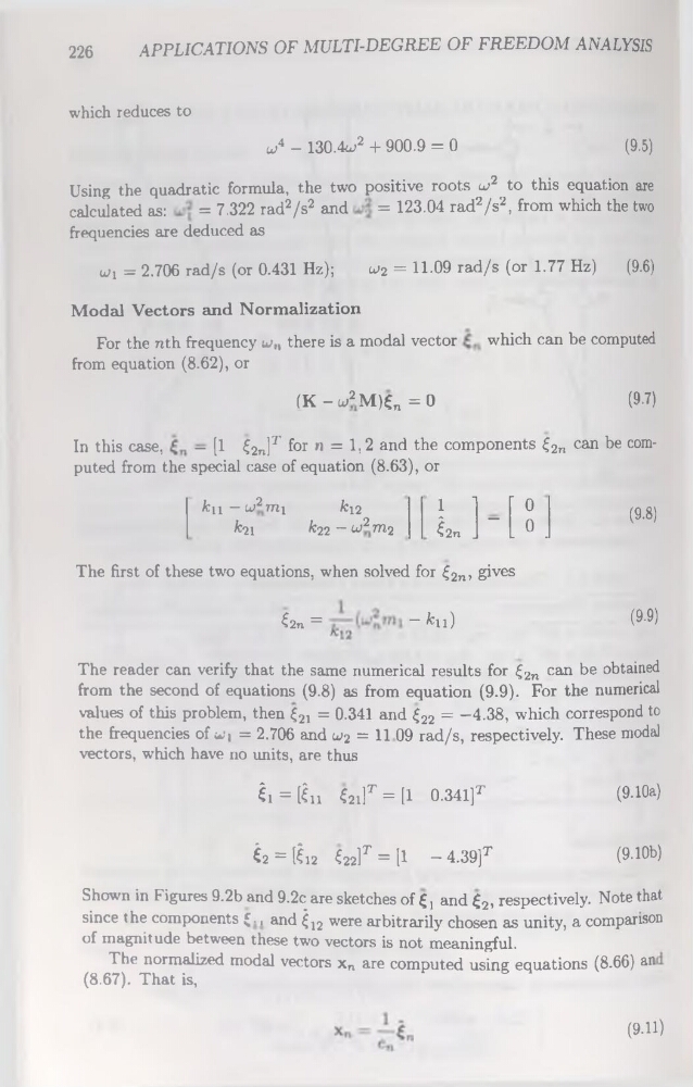
For the nth frequency u>n there is a modal vector
which can be computed
from équation (8.62), or
(K-W2M)Çn =0
(9.7)
In this case,
— [1 £2n]T for n = 1,2 and the components £2n can be computed from the spécial case of équation (8.63), or
I 1 1 F 0
Lu - w2mi
^21
fcl2
fc22 - W2 m2
ê2„ J"L0.
(9.8)
The first of these two équations, when solved for £2n, gives
Gn =
“ M
(9-9)
The reader can verify that the same numerical results for £2n can be obtained
from the second of équations (9.8) as from équation (9.9). For the numerical
values of this problem, then £21 = 0.341 and £22 = —4.38, which correspond to
the frequencies of u'i = 2.706 and cj2 = 1109 rad/s, respectively. These modal
vectors, which hâve no units, are thus
£i = [ên Gi]T = [1 0.341]t
(9.10a)
ê2 = [ê12 <22]T = [1 — 4.39]t
(9.Wb)
Shown in Figures 9.2b and 9.2c are sketches of £ j and £2, respectively. Note that
since the components (•, and £12 were arbitrarily chosen as unity, a comparison
of magnitude between these two vectors is not meaningful.
The normalized modal vectors xn are computed using équations (8-66) an
(8.67). That is,
(9.11)
APPLICATIONS OF MULTI-DEGREE OF FREEDOM ANALYSIS
which reduces to
w4 - 130.4a;2 + 900.9 = 0
(9.5)
Using the quadratic formula, the two positive roots iv2 to this équation are
calculated as:
= 7.322 rad2/s2 and
= 123.04 rad2/s2, from which the two
frequencies are deduced as
uq = 2.706 rad/s (or 0.431 Hz);
w2 = 11.09 rad/s (or 1.77 Hz)
(9.6)
Modal Vectors and Normalization
For the nth frequency u>n there is a modal vector
which can be computed
from équation (8.62), or
(K-W2M)Çn =0
(9.7)
In this case,
— [1 £2n]T for n = 1,2 and the components £2n can be computed from the spécial case of équation (8.63), or
I 1 1 F 0
Lu - w2mi
^21
fcl2
fc22 - W2 m2
ê2„ J"L0.
(9.8)
The first of these two équations, when solved for £2n, gives
Gn =
“ M
(9-9)
The reader can verify that the same numerical results for £2n can be obtained
from the second of équations (9.8) as from équation (9.9). For the numerical
values of this problem, then £21 = 0.341 and £22 = —4.38, which correspond to
the frequencies of u'i = 2.706 and cj2 = 1109 rad/s, respectively. These modal
vectors, which hâve no units, are thus
£i = [ên Gi]T = [1 0.341]t
(9.10a)
ê2 = [ê12 <22]T = [1 — 4.39]t
(9.Wb)
Shown in Figures 9.2b and 9.2c are sketches of £ j and £2, respectively. Note that
since the components (•, and £12 were arbitrarily chosen as unity, a comparison
of magnitude between these two vectors is not meaningful.
The normalized modal vectors xn are computed using équations (8-66) an
(8.67). That is,
(9.11)