

STRUCTURAL RESPONSE STATISTICS: PART II
187
with which équation (7.91) becomes
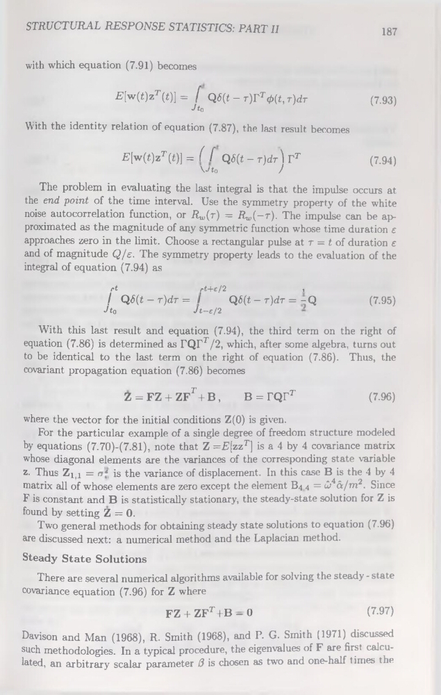
E[w(t)zr(t)] = [ Q6(t - r)rT
J to
With the identity relation of équation (7.87), the last resuit becomes
E[w(t)zT (t)] = ( f Q<5(t - T)dr ) Tt
(7.94)
Vto
/
The problem in evaluating the last intégral is that the impulse occurs at
the end point of the time interval. Use the symmetry property of the white
noise autocorrélation function, or Rw(r) = Rm(—t). The impulse can be approximated as the magnitude of any symmetric function whose time duration e
approaches zéro in the limit. Choose a rectangular puise at t = t of duration e
and of magnitude Q/e. The symmetry property leads to the évaluation of the
intégral of équation (7.94) as
ri
rt+e/2
,
/ Q<5(t - r)dr =
Q<5(t - r)dr = -Q
(7.95)
Jto
Jt-e/2
’
With this last resuit and équation (7.94), the third term on the right of
équation (7.86) is determined as TQrr/2, which, after some algebra, turns out
to be identical to the last term on the right of équation (7.86). Thus, the
covariant propagation équation (7.86) becomes
Z = FZ + ZFr+B,
B = FQFr
(7.96)
where the vector for the initial conditions Z(0) is given.
For the particular example of a single degree of freedom structure modeled
by équations (7.70)-(7.81), note that Z =E[zzr] is a 4 by 4 covariance matrix
whose diagonal éléments are the variances of the corresponding State variable
z. Thus Zj j = rf is the variance of displacement. In this case B is the 4 by 4
matrix ail of whose éléments are zéro except the element B4 4 = Cj^â/m2. Since
F is constant and B is statistically stationary, the steady-state solution for Z is
found by setting Z = 0.
Two general methods for obtaining steady State solutions to équation (7.96)
are discussed next: a numerical method and the Laplacian method.
Steady State Solutions
There are several numerical algorithme available for solving the steady - State
covariance équation (7.96) for Z where
FZ + ZFt+B - 0
(7.97)
Davison and Man (1968), R. Smith (1968), and P. G. Smith (1971) discussed
such méthodologies. In a typical procedure, the eigenvalues of F are first calculated, an arbitrary scalar parameter 3 is chosen as two and one-half times the
187
with which équation (7.91) becomes
E[w(t)zr(t)] = [ Q6(t - r)rT
J to
With the identity relation of équation (7.87), the last resuit becomes
E[w(t)zT (t)] = ( f Q<5(t - T)dr ) Tt
(7.94)
Vto
/
The problem in evaluating the last intégral is that the impulse occurs at
the end point of the time interval. Use the symmetry property of the white
noise autocorrélation function, or Rw(r) = Rm(—t). The impulse can be approximated as the magnitude of any symmetric function whose time duration e
approaches zéro in the limit. Choose a rectangular puise at t = t of duration e
and of magnitude Q/e. The symmetry property leads to the évaluation of the
intégral of équation (7.94) as
ri
rt+e/2
,
/ Q<5(t - r)dr =
Q<5(t - r)dr = -Q
(7.95)
Jto
Jt-e/2
’
With this last resuit and équation (7.94), the third term on the right of
équation (7.86) is determined as TQrr/2, which, after some algebra, turns out
to be identical to the last term on the right of équation (7.86). Thus, the
covariant propagation équation (7.86) becomes
Z = FZ + ZFr+B,
B = FQFr
(7.96)
where the vector for the initial conditions Z(0) is given.
For the particular example of a single degree of freedom structure modeled
by équations (7.70)-(7.81), note that Z =E[zzr] is a 4 by 4 covariance matrix
whose diagonal éléments are the variances of the corresponding State variable
z. Thus Zj j = rf is the variance of displacement. In this case B is the 4 by 4
matrix ail of whose éléments are zéro except the element B4 4 = Cj^â/m2. Since
F is constant and B is statistically stationary, the steady-state solution for Z is
found by setting Z = 0.
Two general methods for obtaining steady State solutions to équation (7.96)
are discussed next: a numerical method and the Laplacian method.
Steady State Solutions
There are several numerical algorithme available for solving the steady - State
covariance équation (7.96) for Z where
FZ + ZFt+B - 0
(7.97)
Davison and Man (1968), R. Smith (1968), and P. G. Smith (1971) discussed
such méthodologies. In a typical procedure, the eigenvalues of F are first calculated, an arbitrary scalar parameter 3 is chosen as two and one-half times the