

170
STATISTICAL RESPONSES FOR LINEAR STRUCTURES
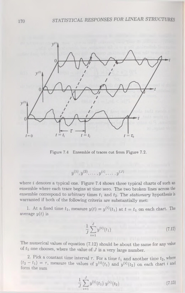
Figure 7.4 Ensemble of traces eut from Figure 7.2.
........ !?'>......... »
ensemble where each trace begins at time zéro. The two broken lines across the
ensemble correspond to arbitrary times G and <2- The stationary hypothesisis
warranted if both of the following criteria are substantially met:
1. At a fixed time tj, measure y{t) = y^(t\) at t — ti on each chart. The
average y(t) is
7 £»"’(«. )
(7.12)
■ 1=1
1 he numerical values of équation (7.12) should be about the saine for any value
of one chooses, where the value of J is a very large number.
2. Pick a constant time interval r. For a time and another time t2, where
(«2 - «i) = r, measure the values of y&(ti) and yV>(t2) on each chart i and
form the sum
1 <
‘
i=l
(7.13)
STATISTICAL RESPONSES FOR LINEAR STRUCTURES
Figure 7.4 Ensemble of traces eut from Figure 7.2.
........ !?'>......... »
ensemble where each trace begins at time zéro. The two broken lines across the
ensemble correspond to arbitrary times G and <2- The stationary hypothesisis
warranted if both of the following criteria are substantially met:
1. At a fixed time tj, measure y{t) = y^(t\) at t — ti on each chart. The
average y(t) is
7 £»"’(«. )
(7.12)
■ 1=1
1 he numerical values of équation (7.12) should be about the saine for any value
of one chooses, where the value of J is a very large number.
2. Pick a constant time interval r. For a time and another time t2, where
(«2 - «i) = r, measure the values of y&(ti) and yV>(t2) on each chart i and
form the sum
1 <
‘
i=l
(7.13)