

134
SINGLE DEGREE OF FREEDOM STRUCTURES
(c) CABLE STRETCH M0DEL
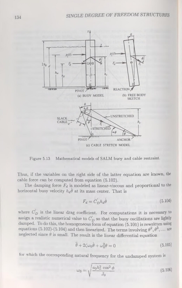
Figure 5.13 Mathematical models of SALM buoy and cable restraint.
Thus, if the variables on the right side of the latter équation are known, the
cable force can be computed from équation (5.102).
The damping force Fd is modeled as linear-viscous and proportional to the
horizontal buoy velocity hd9 at its mass center. That is
Fd — CDhd0
(5.104)
where CD is the linear drag coefficient. For computations it is necessary to
assign a realistic numerical value to CD so that the buoy oscillations are lightly
damped. To do this, the homogeneous form of équation (5.101) is rewritten using
équations (5.102)-(5.104) and then linearized. The terms involving 02,9^, ■ • ■ aje
neglected since 9 is small. The resuit is the linear differential équation
9 +
-b
= 0
(5.105)
for which the corresponding natural frequency for the undamped System is
/ aQh^ cos2 d)
- \---------------V Jo
(5.106)
SINGLE DEGREE OF FREEDOM STRUCTURES
(c) CABLE STRETCH M0DEL
Figure 5.13 Mathematical models of SALM buoy and cable restraint.
Thus, if the variables on the right side of the latter équation are known, the
cable force can be computed from équation (5.102).
The damping force Fd is modeled as linear-viscous and proportional to the
horizontal buoy velocity hd9 at its mass center. That is
Fd — CDhd0
(5.104)
where CD is the linear drag coefficient. For computations it is necessary to
assign a realistic numerical value to CD so that the buoy oscillations are lightly
damped. To do this, the homogeneous form of équation (5.101) is rewritten using
équations (5.102)-(5.104) and then linearized. The terms involving 02,9^, ■ • ■ aje
neglected since 9 is small. The resuit is the linear differential équation
9 +
-b
= 0
(5.105)
for which the corresponding natural frequency for the undamped System is
/ aQh^ cos2 d)
- \---------------V Jo
(5.106)