

RESPONSE FUNCTIONS FOR LINEAR STRUCTURES
119
This value of A(0) must be compatible with équations (5.69) and (5.68). This
is accomplished by integrating équation (5.69) term by term over the impulse
time £, the interval from t = 0“ to t = 0+, or
mh(e) + ci/i(e) + ki
h(t)dt =
6(t)dt
Jo(5.73)
As e —> 0, the right side of the last équation approaches unity by définition,
équation (5.68);
—♦ 0 since the System is not displaced initially, and the
intégral on the left side vanishes. Thus h = 1/m. With équation (5.72), C3 =
l/(ma>d), and with équation (5.70) the solution for the unit impulsive force
becomes
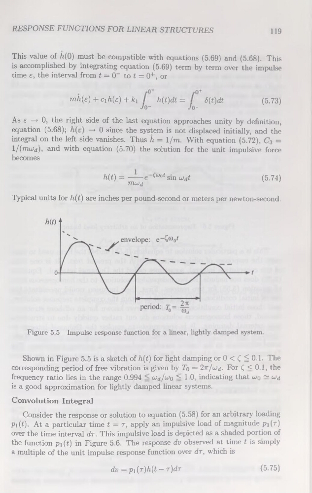
h(t) =------e <>Wo*sin cjrft
mujd
(5.74)
Typical units for h(t) are inches per pound-second or meters per newton-second.
Shown in Figure 5.5 is a sketch of h(t) for light damping or 0 < Ç ^0.1. The
corresponding period of free vibration is given by To = lTT/
is a good approximation for lightly damped linear Systems.
Convolution Intégral
Consider the response or solution to équation (5.58) for an arbitrary loading
Pi(t). At a particular time t — r, apply an impulsive load of magnitude pi(r)
over the time interval dr. This impulsive load is depicted as a shaded portion of
the function pi(t) in Figure 5.6. The response dv observed at time t is simply
a multiple of the unit impulse response function over dr, which is
dv =pi(r)/i(t - r)dr
(5.75)
119
This value of A(0) must be compatible with équations (5.69) and (5.68). This
is accomplished by integrating équation (5.69) term by term over the impulse
time £, the interval from t = 0“ to t = 0+, or
mh(e) + ci/i(e) + ki
h(t)dt =
6(t)dt
Jo(5.73)
As e —> 0, the right side of the last équation approaches unity by définition,
équation (5.68);
—♦ 0 since the System is not displaced initially, and the
intégral on the left side vanishes. Thus h = 1/m. With équation (5.72), C3 =
l/(ma>d), and with équation (5.70) the solution for the unit impulsive force
becomes
h(t) =------e <>Wo*sin cjrft
mujd
(5.74)
Typical units for h(t) are inches per pound-second or meters per newton-second.
Shown in Figure 5.5 is a sketch of h(t) for light damping or 0 < Ç ^0.1. The
corresponding period of free vibration is given by To = lTT/
is a good approximation for lightly damped linear Systems.
Convolution Intégral
Consider the response or solution to équation (5.58) for an arbitrary loading
Pi(t). At a particular time t — r, apply an impulsive load of magnitude pi(r)
over the time interval dr. This impulsive load is depicted as a shaded portion of
the function pi(t) in Figure 5.6. The response dv observed at time t is simply
a multiple of the unit impulse response function over dr, which is
dv =pi(r)/i(t - r)dr
(5.75)