

Fig. 6.3.1.) We are currently in the process of
estimating the Excess CO 2 transport across the
sections shown in Fig. 6.3.12 in order that the
transport distribution in the preindustrial ocean
can be estimated.
Comparisons with earlier budgets and models
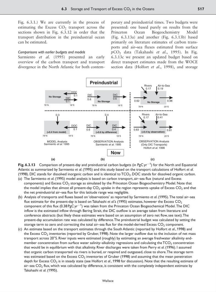
Sarmiento et al. (1995) presented an early
overview of the carbon transport and transport
divergence in the North Atlantic for both contemporary and preindustrial times. Two budgets were
presented: one based purely on results from the
Princeton
Ocean
Biogeochemistry
Model
(Fig. 6.3.13a) and another (Fig. 6.3.13b) based
primarily on literature estimates of carbon transports and air–sea fluxes estimated from surface
pCO 2 data (Takahashi et al., 1995). In Fig.
6.3.13c we present an updated budget based on
direct transport estimates made from the WOCE
section data (Holfort et al., 1998), and storage
6.3 Storage and Transport of Excess CO 2 in the Oceans
517
Wallace
Preindustrial
Now
0.19
0.98
0.62
0.17
Rivers
OBSERVATION Analysis
OBSERVATION Analysis
(Only DIC Transports)
Holfort et al. 1998
0.81
0.63
0.41
Sarmiento et al. 1995
Sarmiento et al. 1995
MODEL Analysis
0.3
0.1
18°S
78°N
18°S
78°N
20°S
78°N
20°S
78°N
18°S
78°N
18°S
78°N
0.1
No Storage
0.1
DOC
DOC
DIC
DIC
DIC
0.4
0.6
0.4
0.6
0.6
(a)
(b)
(c)
DIC
DIC
No Storage
No Storage
(+0.4 from model)
(+0.4 by observation)
(+0.6 by difference)
Air-to-Sea
0.17
Rivers
Air-to-Sea
Fig. 6.3.13 Comparison of present-day and preindustrial carbon budgets (in PgC yr
91
) for the North and Equatorial
Atlantic as summarized by Sarmiento et al. (1995) and this study based on the transport calculations of Holfort et al.
(1998). DIC stands for dissolved inorganic carbon and is identical to TCO 2 . DOC stands for dissolved organic carbon.
(a) The Sarmiento et al. (1995) model analysis is based on carbon transport, air–sea flux (natural and Excess
components) and Excess CO 2 storage as simulated by the Princeton Ocean Biogeochemistry Model. Note that
the model implies that almost all present-day CO 2 uptake in the region represents uptake of Excess CO 2 and that
the net preindustrial air–sea flux for this latitude range was negligible.
(b) Analysis of transports and fluxes based on ‘observations’ as reported by Sarmiento et al. (1995). The total air–sea
flux estimate for the present-day is based on Takahashi et al.’s (1995) estimates, however the Excess CO 2
component of this flux (0.38 PgC yr
91 ) was taken from the Princeton Ocean Biogeochemical Model. The DIC
inflow is the estimated inflow through Bering Strait, the DIC outflow is an average taken from literature and
conference abstracts (but likely these estimates were based on an assumption of zero net flow, see text).The
present-day accumulation rate was calculated by difference.The preindustrial budget was calculated by setting the
storage term to zero and correcting the total air–sea flux for the model-derived Excess CO 2 component.
(c) An estimate based on the transport estimates through the South Atlantic (reported by Holfort et al., 1998) and
the Excess CO 2 inventories (reported by Gruber, 1998). Note the larger outflow due to the inclusion of net mass
transport across 20°S. River inputs were estimated (roughly) by estimating an average freshwater alkalinity endmember concentration from surface water salinity–alkalinity regressions and calculating the TCO 2 concentration
that would be in equilibrium with that alkalinity. River discharges were taken from Perry et al. (1996). I assumed
that organic carbon transported via rivers is buried, or respired and outgassed, close to shore.The storage term
was estimated based on the Excess CO 2 inventories of Gruber (1998) and assuming that the mean penetration
depth for Excess CO 2 is in steady state (see Holfort et al., 1998 for discussion). Note that the resulting estimate of
air–sea CO 2 flux, which was calculated by difference, is consistent with the completely independent estimate by
Takahashi et al. (1995).
estimating the Excess CO 2 transport across the
sections shown in Fig. 6.3.12 in order that the
transport distribution in the preindustrial ocean
can be estimated.
Comparisons with earlier budgets and models
Sarmiento et al. (1995) presented an early
overview of the carbon transport and transport
divergence in the North Atlantic for both contemporary and preindustrial times. Two budgets were
presented: one based purely on results from the
Princeton
Ocean
Biogeochemistry
Model
(Fig. 6.3.13a) and another (Fig. 6.3.13b) based
primarily on literature estimates of carbon transports and air–sea fluxes estimated from surface
pCO 2 data (Takahashi et al., 1995). In Fig.
6.3.13c we present an updated budget based on
direct transport estimates made from the WOCE
section data (Holfort et al., 1998), and storage
6.3 Storage and Transport of Excess CO 2 in the Oceans
517
Wallace
Preindustrial
Now
0.19
0.98
0.62
0.17
Rivers
OBSERVATION Analysis
OBSERVATION Analysis
(Only DIC Transports)
Holfort et al. 1998
0.81
0.63
0.41
Sarmiento et al. 1995
Sarmiento et al. 1995
MODEL Analysis
0.3
0.1
18°S
78°N
18°S
78°N
20°S
78°N
20°S
78°N
18°S
78°N
18°S
78°N
0.1
No Storage
0.1
DOC
DOC
DIC
DIC
DIC
0.4
0.6
0.4
0.6
0.6
(a)
(b)
(c)
DIC
DIC
No Storage
No Storage
(+0.4 from model)
(+0.4 by observation)
(+0.6 by difference)
Air-to-Sea
0.17
Rivers
Air-to-Sea
Fig. 6.3.13 Comparison of present-day and preindustrial carbon budgets (in PgC yr
91
) for the North and Equatorial
Atlantic as summarized by Sarmiento et al. (1995) and this study based on the transport calculations of Holfort et al.
(1998). DIC stands for dissolved inorganic carbon and is identical to TCO 2 . DOC stands for dissolved organic carbon.
(a) The Sarmiento et al. (1995) model analysis is based on carbon transport, air–sea flux (natural and Excess
components) and Excess CO 2 storage as simulated by the Princeton Ocean Biogeochemistry Model. Note that
the model implies that almost all present-day CO 2 uptake in the region represents uptake of Excess CO 2 and that
the net preindustrial air–sea flux for this latitude range was negligible.
(b) Analysis of transports and fluxes based on ‘observations’ as reported by Sarmiento et al. (1995). The total air–sea
flux estimate for the present-day is based on Takahashi et al.’s (1995) estimates, however the Excess CO 2
component of this flux (0.38 PgC yr
91 ) was taken from the Princeton Ocean Biogeochemical Model. The DIC
inflow is the estimated inflow through Bering Strait, the DIC outflow is an average taken from literature and
conference abstracts (but likely these estimates were based on an assumption of zero net flow, see text).The
present-day accumulation rate was calculated by difference.The preindustrial budget was calculated by setting the
storage term to zero and correcting the total air–sea flux for the model-derived Excess CO 2 component.
(c) An estimate based on the transport estimates through the South Atlantic (reported by Holfort et al., 1998) and
the Excess CO 2 inventories (reported by Gruber, 1998). Note the larger outflow due to the inclusion of net mass
transport across 20°S. River inputs were estimated (roughly) by estimating an average freshwater alkalinity endmember concentration from surface water salinity–alkalinity regressions and calculating the TCO 2 concentration
that would be in equilibrium with that alkalinity. River discharges were taken from Perry et al. (1996). I assumed
that organic carbon transported via rivers is buried, or respired and outgassed, close to shore.The storage term
was estimated based on the Excess CO 2 inventories of Gruber (1998) and assuming that the mean penetration
depth for Excess CO 2 is in steady state (see Holfort et al., 1998 for discussion). Note that the resulting estimate of
air–sea CO 2 flux, which was calculated by difference, is consistent with the completely independent estimate by
Takahashi et al. (1995).