

levels for this time period has been plotted assuming surface waters in this region have maintained
equilibrium with respect to the increasing atmospheric pCO 2 . Both Excess CO 2 estimates deviate
significantly from the theoretical values in the
upper layers: this may reflect problems with calculating Excess CO 2 levels in the upper ocean using
summertime data (see Section 6.3.4.1). Uncertainties in the upper 200 m of the water column can
therefore be significant.
To date no comprehensive analysis of the
Atlantic Ocean CO 2 data collected during WOCE
has been conducted, although this is being planned
(e.g. Mintrop and Wallace, 1999). However, based
on Gruber’s (1998) analysis, the North Atlantic
Ocean contained a total of about 22<5 PgC of
Excess CO 2 in 1982 and the South Atlantic contained about 18<4 PgC Excess CO 2 in 1989. The
stated uncertainty is larger than the estimated
effect of purely random errors due to the possible
effect of systematic error when calculating inventories (see Gruber (1998) and the discussion
above). The global inventories of oceanic Excess
CO 2 (all oceans) predicted by the Princeton Ocean
Biogeochemistry Model were 106 PgC (1982) and
120 PgC (1989). Simple scaling of the basin-scale
estimates by this modelled temporal increase of the
global inventory implies a total Atlantic Ocean
inventory of about 43 PgC for the year 1989.
Indian Ocean
Sabine et al. (1999) performed a comprehensive
analysis of the basin-wide inventory of Excess CO 2
based on data collected during the US WOCE Survey of the Indian Ocean (December 1994 through
January 1996). Data from nine US WOCE legs
were used together with data from I6S collected
during the French CIVA1 cruise and some preWOCE data from the Southwestern Indian Ocean.
Two separate methods were used to examine
Excess CO 2 : a time-series comparison with data
collected two decades earlier during GEOSECS
(see Section 6.3.4.2) and a slightly modified version of Gruber’s ⌬C
* technique.
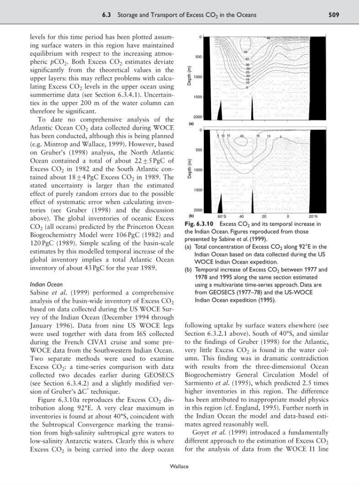
Figure 6.3.10a reproduces the Excess CO 2 distribution along 92°E. A very clear maximum in
inventories is found at about 40°S, coincident with
the Subtropical Convergence marking the transition from high-salinity subtropical gyre waters to
low-salinity Antarctic waters. Clearly this is where
Excess CO 2 is being carried into the deep ocean
following uptake by surface waters elsewhere (see
Section 6.3.2.1 above). South of 40°S, and similar
to the findings of Gruber (1998) for the Atlantic,
very little Excess CO 2 is found in the water column. This finding was in dramatic contradiction
with results from the three-dimensional Ocean
Biogeochemistry General Circulation Model of
Sarmiento et al. (1995), which predicted 2.5 times
higher inventories in this region. The difference
has been attributed to inappropriate model physics
in this region (cf. England, 1995). Further north in
the Indian Ocean the model and data-based estimates agreed reasonably well.
Goyet et al. (1999) introduced a fundamentally
different approach to the estimation of Excess CO 2
for the analysis of data from the WOCE I1 line
6.3 Storage and Transport of Excess CO 2 in the Oceans
509
Wallace
60°S
4 0
2 0
2 0 °N
2000
1500
1000
500
0
.
.
.
5
10
15
15
20
.
.
.
.
.
.
.
.
.
.
.
.
.
.
. .
.
.
.
.
.
.
.
.
.
.
.
.
.
.
.
.
.
.
.
.
.
.
.
.
.
.
.
.
.
.
.
.
.
.
.
.
.
.
.
.
.
.
.
.
.
.
.
.
.
.
.
.
.
.
.
.
.
.
.
.
.
.
.
.
.
.
.
.
.
.
.
.
.
.
.
.
.
.
.
.
.
.
.
.
.
.
.
.
.
.
.
.
.
.
.
.
.
.
.
.
.
.
.
.
.
.
.
.
.
.
.
.
.
.
.
.
.
.
.
.
.
.
.
.
.
.
.
.
.
.
.
.
.
.
.
.
.
.
.
.
.
.
.
.
.
.
.
.
.
.
.
.
.
.
.
.
.
.
.
.
.
.
.
.
.
.
.
.
.
.
.
.
.
.
.
.
.
.
.
.
.
.
.
.
.
.
.
.
.
.
.
.
.
.
.
.
.
.
.
.
.
.
.
.
.
.
.
.
.
.
.
.
.
.
.
.
.
.
.
.
.
.
.
.
.
.
.
.
.
.
.
.
.
.
.
.
.
.
.
.
.
.
.
. .
.
.
.
.
.
.
.
.
.
.
.
.
.
.
.
.
.
.
.
.
.
.
.
.
.
.
.
.
.
.
.
.
.
.
.
.
.
.
.
.
.
.
.
.
.
.
.
.
.
.
.
.
.
.
.
.
.
.
.
.
.
.
.
.
.
.
.
.
.
.
.
.
.
.
.
.
.
.
.
.
.
.
.
.
.
.
.
.
.
.
.
.
.
.
.
.
.
.
.
.
.
.
.
.
.
.
.
.
.
.
.
.
.
.
.
.
.
.
.
.
.
.
.
.
.
.
.
.
.
.
.
.
.
.
.
.
.
.
.
.
.
.
.
.
.
.
.
.
.
.
.
.
.
.
.
.
.
.
.
.
.
.
.
.
.
.
.
.
.
.
.
.
.
.
.
.
.
.
.
.
.
.
.
.
.
.
.
.
.
.
.
.
.
.
.
.
.
.
.
.
.
.
.
.
.
.
.
.
.
.
.
.
.
.
.
.
.
.
.
.
.
.
.
.
.
. .
.
.
.
.
.
. .
.
.
.
. .
.
.
.
.
.
.
.
.
.
.
.
.
.
.
.
. .
. .
..
.
.
.
.
.
.
.
.
.
.
.
.
.
.
.
.
.
...
.
.
.
.
.
.
.
.
.
.
.
.
.
.
.
.
.
.
.
.
.
.. . .
.
.
.
.
.
.
.
.
.
.
.
.
.
.
.. .
. .
.
.
.
.
.
.
.
.
.
.
..
.
.
.
.
.
.
.
.
.
.
.
.
.
.
.
..
. .
.
.
.
.
.
.
.
.
.
.
.
.
.
..
.
.
.
.
.
.
.
.
.
.
.
.
.
.
.
..
.
. .
.
.
.
.
.
.
.
.
.
.
.
.
.
.. .
.
.
.
.
.
.
.
.
.
.
.
.
.
..
. .
.
.
.
.
.
.
.
.
.
.
.
.
.
.
.. .
.
.
.
.
.
.
.
.
.
.
.
.
.
..
.
.
.
.
.
.
.
.
.
.
.
.
.
.
.
.
.
.
.
.
.
.
.
.
.
.
..
.
.
.
.
. .
.
.
.
.
.
.
.
.
..
.
.
.
.
.
.
.
.
.
.
.
..
.
.
.
.
.
.
.
.
.
.
.
.
.
.
.
.
.
..
.
.
.
.
. .
.
.
.
.
.
.
.
.
.
.
.
..
.
.
.
.
.
.
.
.
.
.
.
.
.
...
. . .
. . .
. .
.
.
.
.
.
.
.
.
.
. .
.
.
.
.
.
.
.
.
.
.
.
.
.
.. .
.
.
.
.
.
.
.
.
.
.
.
.
.
..
.
.
.
.
.
.
.
.
.
.
.
.
.
...
.
.
.
.
.
.
.
.
.
.
.
.
.
..
.
.
.
.
.
.
.
.
.
.
.
.
.
.
.
.
..
.
. .
.
.
.
.
.
.
.
.
.
.
.
.. .
.
.
.
.
.
.
.
.
.
.
.
.
.
.
.
.
.
..
. . .
.
.
.
.
.
.
.
. .
.
.
.
.. .
.
.
.
.
.
.
.
.
.
.
.
.
.
..
.
.
.
.
.
. .
.
.
.
.
.
.
.
.
.
..
.
.
.
. .
.
.
.
.
.
.
.
.
.
.
.
.
.
..
. . . . .
.
. .
.
.
.
.. .
..
. . .
.
.
.
.
.
.
.
.
.
.
..
.
.
.
.
.
.
.
.
.
.
.
.
.
.
.
.
.
.. .
.
.
.
..
.
. .
.
.
.
.
.
.
.
.
.. .
.
.
.
.
.
.
.
.
.
.
.
.
.
.
..
.
. .
.
.
.
.
.
.
.
.
.
.
.. .
.
.
.
.
.
.
.
.
.
.
.
.
.
.
.
.
..
. . .
.
.
.
.
. .
.
.
.
.
.
.
.
.
.
.
.
.
.
.
.
.
.
.
.
.
.
.
.
.
. . .
.
.
.
.
.
.
.
.
.
.
.
.
.
..
.
.
.
.
.
.
.
.
.
.
.
.
.
.
.
.
.
.
.
..
. .
.
.
.
.
.
.
.
.
.
.
.
..
.
.
.
.
.
.
.
.
.
.
.
..
. .
.
.
.
.
.
.
.
.
.
. .
.
.
.
.
.
...
.
.
.
.
.
.
.
.
.
.
.
.
.
.
.
.
.
.
.
.
...
. .
..
. . .
.
.
.
.
.
.
.
.
.
.
...
.
.
.
.
.
.
.
.
.
.
.
.
.
.
.
.
..
.
.
.
.
.
.
.
.
.
.
.
.
.
.
.
.
.
.
.. .
.
.
. .
.
. .
.
. . .
.
.
.
.
.
.
.
..
.
.
.
.
.
.
.
.
.
.
.
.
.
.
.
.
.
.
..
.
.
.
.
. .
.
.
.
.
.
.
.
.
.
.
.
.
.
.
.
.
.
.
.
.
.
.
.
.
.
.
.
.
.
Depth (m)
5 10
2000
1500
1000
500
0
Depth (m)
. . . .
.
.
.
.
.
.
5
10
15
20
25
30
35
40
45
45
. .
.
.
.
.
.
.
.
.
.
.
.
.
.
.
.
.
. . . . .
.
.
.
.
.
.
.
.
.
.
.
.
.
.
.
.
.
.
. .
.
.
.
.
.
.
.
.
.
.
.
.
.
.
.
.
. . . .
.
.
.
.
.
.
.
.
.
.
.
.
. . .
.
.
.
.
.
.
.
.
.
.
.
.
.
.
.
.
. .
. .
.
.
.
.
.
.
.
.
.
.
.
.
.
.
.
.
.
.
.
.
. .
. .
.
.
.
.
.
.
.
.
.
.
.
.
. .
. .
.
.
.
.
.
.
.
.
.
.
.
.
.
.
.
.
.
.
.
.
.
.
.
.
.
.
.
.
.
.
.
.
.
.
.
. .
.
.
.
.
.
.
.
.
.
.
.
.
.
.
.
. . . .
.
.
.
.
.
.
.
.
.
.
.
.
.
.
.
.
.
.
.
.
.
.
.
.
.
.
.
.
.
.
.
.
.
.
.
.
.
.
.
.
.
.
.
.
.
.
.
.
.
.
.
.
.
.
.
.
.
.
.
.
.
.
. . .
.
.
.
.
.
.
.
.
.
.
.
.
.
.
.
.
.
.
.
.
.
.
.
.
.
.
.
.
.
.
. . .
.
.
.
.
.
.
.
.
.
.
.
.
.
.
.
.
.
.
.
.
.
.
.
.
.
.
.
.
.
.
.
.
.
.
.
.
.
.
.
.
.
.
.
.
.
.
.
.
.
.
. . .
.
.
.
.
.
.
.
.
.
.
.
.
.
.
.
.
.
.
. .
.
.
.
.
.
.
.
.
.
.
.
.
.
.
.
.
.
.
.
.
.
.
.
.
.
.
.
.
.
.
.
.
.
.
.
.
.
.
.
.
.
.
.
.
.
.
.
.
.
.
.
.
. . .
.
.
.
.
.
.
.
.
.
.
.
.
. .
.
.
.
.
.
.
.
.
.
.
.
.
.
.
.
.
.
.
.
. . .
.
.
.
.
.
.
.
.
.
.
.
.
.
.
.
.
.
.
.
.
.
.
.
.
.
.
.
.
.
.
.
.
.
.
.
.
.
.
.
.
.
.
.
.
.
.
.
.
.
.
.
.
.
.
.
.
.
.
.
.
.
.
.
.
. . .
.
.
.
.
.
.
.
.
.
.
.
.
.
.
.
.
.
.
.
.
.
.
.
. .
.
.
.
.
.
. .
.
.
.
.
. .
.
.
.
.
.
.
.
.
.
.
.
.
.
.
. .
.
.
.
.
.
.
.
.
.
.
.
.
.
.
.
.
.
.
.
.
.
.
.
.
.
.
.
.
.
.
.
.
.
.
.
.
.
.
.
.
.
.
.
.
.
.
.
.
.
.
.
.
.
.
.
.
.
.. . .
. .
.
. .
.
.
.
.
.
.
.
.
.
.
.
.
.
.
.
.
.
.
.
.
.
.
.
.
.
.
.
..
.
. . .
.
.
.
.
.
.
.
.
.
.
.
.
.
.
.
..
.
.
.
.
.
.
.
.
.
.
.
.
.
.
.
.
..
.
.
.
. .
.
.
.
.
.
.
.
.
.
.
.
.
.
.
..
.
.
.
.
.
.
.
.
.
.
.
.
.
.
. . .
. .
.
.
.
.
.
.
.
.
.
.
.
.
.
.
.
..
.
.
.
.
.
.
.
.
.
.
.
.
.
.
.
.. .
. . .
.
.
.
.
.
.
.
.
.
.
.
.
.
. .
. .
.
.
.
.
.
.
.
.
.
.
.
.
.
..
. . .
. .
.
.
.
.
. .
.
.
.
.
.
.
.
.
.. .
. ..
.
.
.
.
.
.
.
.
.
.
.
.
.
.. .
. .
.
. .
.
.
.
.
.
.
.
.
.
.
.
.
.
.
.
.
.
..
.
. . .
.
.
.
.
. .
.
.
.
.
.
.
.
.
.
.
.
...
..
. .
.
.
.
.
.
.
.
.
.
.
.
.
.
...
.
.
. .
.
. . .
. . .
. .
.
.
.
.
.
.
.
.
.
. . . ..
.
.
.
.
.
.
.
.
.
.
.
.
.
.
.
.. . .
. .
. .
.
.
.
.
.
.
.
.
.
.
.
.
.
.
.
.. . .
..
.
.
.
.
.
.
.
.
.
.
.
.
.
.
.
..
.
.
.
.
.
.
.
.
.
.
.
.
.
.
.
.
.
.
..
.
. .
. .
.
.
.
.
.
.
.
.
.
.
.
.
.
.
.
.
.. . . . . . .
. .
.
. .
.
.
.
.
.
.
.
.
.
.
.
.. . . .
. .
.
.
.
.
.
.
.
.
.
.
.
.
.
.
.
.
.
.. . .
. . .
.
. . .
.
.
.
.
.
.
.
.
.
.
.
.. . . . .
.
.
.
.
.
.
.
.
.
.
.
.
.
.
.
..
.
. .
. .
.
.
.
.
. .
.
.
.
.
.
.
.
.
.
...
..
.
.
.
.
.
. .
.
.
.
.
.
.
.
.
.
.
.
.
.
..
. .
.
.
. . . . .
.
. .
.
.
.
.
.. .
. . . .
..
. . .
.
.
.
.
.
.
.
.
.
.
. . . . .
.
.
.
.
.
.
.
.
.
.
.
.
.
.
.
.
.
.
.. .
. . .
. . .
.
.
..
.
.
. .
.
.
.
.
.
.
.
.
.. . .
.
.
.
.
.
.
.
.
.
.
.
.
.
.
.
.
.
.
. .
. . .
. .
.
. .
.
.
.
.
.
.
.
.
.
.
.. . . . .
.
.
.
.
.
.
.
.
.
.
.
.
.
.
.
.
.
.
..
..
. .
. . .
.
.
.
.
. .
.
.
.
.
.
.
.
.. . ..
.
.
.
.
.
.
.
.
.
.
.
.
.
.
.
.
.
.
..
. . .
.
. . .
.
.
.
.
.
.
.
.
.
.
.
.
.
.. . . . .
.
.
.
.
.
.
.
.
.
.
.
.
.
.
.
.
.
.
.
.
.. . . . .
. .
. .
.
.
.
.
.
.
.
.
.
.
.
.
.
.
.
.
.
.
.
.
.
.
.
.
.
..
. . .
..
. .
.
.
.
.
.
.
.
.
.
. .
.
.
.
.
.
...
. . .
.
.
.
.
.
.
.
.
.
.
.
.
.
.
.
.
.
.
.
.
... . . .
. .
. .
..
. . .
.
.
.
.
.
.
.
.
.
.
..
. . . . .
.
.
.
.
.
.
.
.
.
.
.
.
.
.
.
.
.
. .
.
.
.
.
.
.
.
.
.
.
.
.
.
.
.
.
.
.
.
.
..
.. . . . .
.
.
. .
.
. .
.
. . .
.
.
.
.
.
.
.
...
.
.
.
.
.
.
.
.
.
.
.
.
.
.
.
.
.
. . . . .
.
.
.
.
. .
.
.
.
.
.
.
.
.
.
.
.
.
.
.
.
.
.
.
.
.
.
.
.
.
.
.
.
.
.
.
.
(a)
(b)
0
Fig. 6.3.10 Excess CO 2 and its temporal increase in
the Indian Ocean. Figures reproduced from those
presented by Sabine et al. (1999).
(a) Total concentration of Excess CO 2 along 92°E in the
Indian Ocean based on data collected during the US
WOCE Indian Ocean expedition.
(b) Temporal increase of Excess CO 2 between 1977 and
1978 and 1995 along the same section estimated
using a multivariate time-series approach. Data are
from GEOSECS (1977–78) and the US-WOCE
Indian Ocean expedition (1995).
equilibrium with respect to the increasing atmospheric pCO 2 . Both Excess CO 2 estimates deviate
significantly from the theoretical values in the
upper layers: this may reflect problems with calculating Excess CO 2 levels in the upper ocean using
summertime data (see Section 6.3.4.1). Uncertainties in the upper 200 m of the water column can
therefore be significant.
To date no comprehensive analysis of the
Atlantic Ocean CO 2 data collected during WOCE
has been conducted, although this is being planned
(e.g. Mintrop and Wallace, 1999). However, based
on Gruber’s (1998) analysis, the North Atlantic
Ocean contained a total of about 22<5 PgC of
Excess CO 2 in 1982 and the South Atlantic contained about 18<4 PgC Excess CO 2 in 1989. The
stated uncertainty is larger than the estimated
effect of purely random errors due to the possible
effect of systematic error when calculating inventories (see Gruber (1998) and the discussion
above). The global inventories of oceanic Excess
CO 2 (all oceans) predicted by the Princeton Ocean
Biogeochemistry Model were 106 PgC (1982) and
120 PgC (1989). Simple scaling of the basin-scale
estimates by this modelled temporal increase of the
global inventory implies a total Atlantic Ocean
inventory of about 43 PgC for the year 1989.
Indian Ocean
Sabine et al. (1999) performed a comprehensive
analysis of the basin-wide inventory of Excess CO 2
based on data collected during the US WOCE Survey of the Indian Ocean (December 1994 through
January 1996). Data from nine US WOCE legs
were used together with data from I6S collected
during the French CIVA1 cruise and some preWOCE data from the Southwestern Indian Ocean.
Two separate methods were used to examine
Excess CO 2 : a time-series comparison with data
collected two decades earlier during GEOSECS
(see Section 6.3.4.2) and a slightly modified version of Gruber’s ⌬C
* technique.
Figure 6.3.10a reproduces the Excess CO 2 distribution along 92°E. A very clear maximum in
inventories is found at about 40°S, coincident with
the Subtropical Convergence marking the transition from high-salinity subtropical gyre waters to
low-salinity Antarctic waters. Clearly this is where
Excess CO 2 is being carried into the deep ocean
following uptake by surface waters elsewhere (see
Section 6.3.2.1 above). South of 40°S, and similar
to the findings of Gruber (1998) for the Atlantic,
very little Excess CO 2 is found in the water column. This finding was in dramatic contradiction
with results from the three-dimensional Ocean
Biogeochemistry General Circulation Model of
Sarmiento et al. (1995), which predicted 2.5 times
higher inventories in this region. The difference
has been attributed to inappropriate model physics
in this region (cf. England, 1995). Further north in
the Indian Ocean the model and data-based estimates agreed reasonably well.
Goyet et al. (1999) introduced a fundamentally
different approach to the estimation of Excess CO 2
for the analysis of data from the WOCE I1 line
6.3 Storage and Transport of Excess CO 2 in the Oceans
509
Wallace
60°S
4 0
2 0
2 0 °N
2000
1500
1000
500
0
.
.
.
5
10
15
15
20
.
.
.
.
.
.
.
.
.
.
.
.
.
.
. .
.
.
.
.
.
.
.
.
.
.
.
.
.
.
.
.
.
.
.
.
.
.
.
.
.
.
.
.
.
.
.
.
.
.
.
.
.
.
.
.
.
.
.
.
.
.
.
.
.
.
.
.
.
.
.
.
.
.
.
.
.
.
.
.
.
.
.
.
.
.
.
.
.
.
.
.
.
.
.
.
.
.
.
.
.
.
.
.
.
.
.
.
.
.
.
.
.
.
.
.
.
.
.
.
.
.
.
.
.
.
.
.
.
.
.
.
.
.
.
.
.
.
.
.
.
.
.
.
.
.
.
.
.
.
.
.
.
.
.
.
.
.
.
.
.
.
.
.
.
.
.
.
.
.
.
.
.
.
.
.
.
.
.
.
.
.
.
.
.
.
.
.
.
.
.
.
.
.
.
.
.
.
.
.
.
.
.
.
.
.
.
.
.
.
.
.
.
.
.
.
.
.
.
.
.
.
.
.
.
.
.
.
.
.
.
.
.
.
.
.
.
.
.
.
.
.
.
.
.
.
.
.
.
.
.
.
.
.
.
.
.
.
.
. .
.
.
.
.
.
.
.
.
.
.
.
.
.
.
.
.
.
.
.
.
.
.
.
.
.
.
.
.
.
.
.
.
.
.
.
.
.
.
.
.
.
.
.
.
.
.
.
.
.
.
.
.
.
.
.
.
.
.
.
.
.
.
.
.
.
.
.
.
.
.
.
.
.
.
.
.
.
.
.
.
.
.
.
.
.
.
.
.
.
.
.
.
.
.
.
.
.
.
.
.
.
.
.
.
.
.
.
.
.
.
.
.
.
.
.
.
.
.
.
.
.
.
.
.
.
.
.
.
.
.
.
.
.
.
.
.
.
.
.
.
.
.
.
.
.
.
.
.
.
.
.
.
.
.
.
.
.
.
.
.
.
.
.
.
.
.
.
.
.
.
.
.
.
.
.
.
.
.
.
.
.
.
.
.
.
.
.
.
.
.
.
.
.
.
.
.
.
.
.
.
.
.
.
.
.
.
.
.
.
.
.
.
.
.
.
.
.
.
.
.
.
.
.
.
.
. .
.
.
.
.
.
. .
.
.
.
. .
.
.
.
.
.
.
.
.
.
.
.
.
.
.
.
. .
. .
..
.
.
.
.
.
.
.
.
.
.
.
.
.
.
.
.
.
...
.
.
.
.
.
.
.
.
.
.
.
.
.
.
.
.
.
.
.
.
.
.. . .
.
.
.
.
.
.
.
.
.
.
.
.
.
.
.. .
. .
.
.
.
.
.
.
.
.
.
.
..
.
.
.
.
.
.
.
.
.
.
.
.
.
.
.
..
. .
.
.
.
.
.
.
.
.
.
.
.
.
.
..
.
.
.
.
.
.
.
.
.
.
.
.
.
.
.
..
.
. .
.
.
.
.
.
.
.
.
.
.
.
.
.
.. .
.
.
.
.
.
.
.
.
.
.
.
.
.
..
. .
.
.
.
.
.
.
.
.
.
.
.
.
.
.
.. .
.
.
.
.
.
.
.
.
.
.
.
.
.
..
.
.
.
.
.
.
.
.
.
.
.
.
.
.
.
.
.
.
.
.
.
.
.
.
.
.
..
.
.
.
.
. .
.
.
.
.
.
.
.
.
..
.
.
.
.
.
.
.
.
.
.
.
..
.
.
.
.
.
.
.
.
.
.
.
.
.
.
.
.
.
..
.
.
.
.
. .
.
.
.
.
.
.
.
.
.
.
.
..
.
.
.
.
.
.
.
.
.
.
.
.
.
...
. . .
. . .
. .
.
.
.
.
.
.
.
.
.
. .
.
.
.
.
.
.
.
.
.
.
.
.
.
.. .
.
.
.
.
.
.
.
.
.
.
.
.
.
..
.
.
.
.
.
.
.
.
.
.
.
.
.
...
.
.
.
.
.
.
.
.
.
.
.
.
.
..
.
.
.
.
.
.
.
.
.
.
.
.
.
.
.
.
..
.
. .
.
.
.
.
.
.
.
.
.
.
.
.. .
.
.
.
.
.
.
.
.
.
.
.
.
.
.
.
.
.
..
. . .
.
.
.
.
.
.
.
. .
.
.
.
.. .
.
.
.
.
.
.
.
.
.
.
.
.
.
..
.
.
.
.
.
. .
.
.
.
.
.
.
.
.
.
..
.
.
.
. .
.
.
.
.
.
.
.
.
.
.
.
.
.
..
. . . . .
.
. .
.
.
.
.. .
..
. . .
.
.
.
.
.
.
.
.
.
.
..
.
.
.
.
.
.
.
.
.
.
.
.
.
.
.
.
.
.. .
.
.
.
..
.
. .
.
.
.
.
.
.
.
.
.. .
.
.
.
.
.
.
.
.
.
.
.
.
.
.
..
.
. .
.
.
.
.
.
.
.
.
.
.
.. .
.
.
.
.
.
.
.
.
.
.
.
.
.
.
.
.
..
. . .
.
.
.
.
. .
.
.
.
.
.
.
.
.
.
.
.
.
.
.
.
.
.
.
.
.
.
.
.
.
. . .
.
.
.
.
.
.
.
.
.
.
.
.
.
..
.
.
.
.
.
.
.
.
.
.
.
.
.
.
.
.
.
.
.
..
. .
.
.
.
.
.
.
.
.
.
.
.
..
.
.
.
.
.
.
.
.
.
.
.
..
. .
.
.
.
.
.
.
.
.
.
. .
.
.
.
.
.
...
.
.
.
.
.
.
.
.
.
.
.
.
.
.
.
.
.
.
.
.
...
. .
..
. . .
.
.
.
.
.
.
.
.
.
.
...
.
.
.
.
.
.
.
.
.
.
.
.
.
.
.
.
..
.
.
.
.
.
.
.
.
.
.
.
.
.
.
.
.
.
.
.. .
.
.
. .
.
. .
.
. . .
.
.
.
.
.
.
.
..
.
.
.
.
.
.
.
.
.
.
.
.
.
.
.
.
.
.
..
.
.
.
.
. .
.
.
.
.
.
.
.
.
.
.
.
.
.
.
.
.
.
.
.
.
.
.
.
.
.
.
.
.
.
Depth (m)
5 10
2000
1500
1000
500
0
Depth (m)
. . . .
.
.
.
.
.
.
5
10
15
20
25
30
35
40
45
45
. .
.
.
.
.
.
.
.
.
.
.
.
.
.
.
.
.
. . . . .
.
.
.
.
.
.
.
.
.
.
.
.
.
.
.
.
.
.
. .
.
.
.
.
.
.
.
.
.
.
.
.
.
.
.
.
. . . .
.
.
.
.
.
.
.
.
.
.
.
.
. . .
.
.
.
.
.
.
.
.
.
.
.
.
.
.
.
.
. .
. .
.
.
.
.
.
.
.
.
.
.
.
.
.
.
.
.
.
.
.
.
. .
. .
.
.
.
.
.
.
.
.
.
.
.
.
. .
. .
.
.
.
.
.
.
.
.
.
.
.
.
.
.
.
.
.
.
.
.
.
.
.
.
.
.
.
.
.
.
.
.
.
.
.
. .
.
.
.
.
.
.
.
.
.
.
.
.
.
.
.
. . . .
.
.
.
.
.
.
.
.
.
.
.
.
.
.
.
.
.
.
.
.
.
.
.
.
.
.
.
.
.
.
.
.
.
.
.
.
.
.
.
.
.
.
.
.
.
.
.
.
.
.
.
.
.
.
.
.
.
.
.
.
.
.
. . .
.
.
.
.
.
.
.
.
.
.
.
.
.
.
.
.
.
.
.
.
.
.
.
.
.
.
.
.
.
.
. . .
.
.
.
.
.
.
.
.
.
.
.
.
.
.
.
.
.
.
.
.
.
.
.
.
.
.
.
.
.
.
.
.
.
.
.
.
.
.
.
.
.
.
.
.
.
.
.
.
.
.
. . .
.
.
.
.
.
.
.
.
.
.
.
.
.
.
.
.
.
.
. .
.
.
.
.
.
.
.
.
.
.
.
.
.
.
.
.
.
.
.
.
.
.
.
.
.
.
.
.
.
.
.
.
.
.
.
.
.
.
.
.
.
.
.
.
.
.
.
.
.
.
.
.
. . .
.
.
.
.
.
.
.
.
.
.
.
.
. .
.
.
.
.
.
.
.
.
.
.
.
.
.
.
.
.
.
.
.
. . .
.
.
.
.
.
.
.
.
.
.
.
.
.
.
.
.
.
.
.
.
.
.
.
.
.
.
.
.
.
.
.
.
.
.
.
.
.
.
.
.
.
.
.
.
.
.
.
.
.
.
.
.
.
.
.
.
.
.
.
.
.
.
.
.
. . .
.
.
.
.
.
.
.
.
.
.
.
.
.
.
.
.
.
.
.
.
.
.
.
. .
.
.
.
.
.
. .
.
.
.
.
. .
.
.
.
.
.
.
.
.
.
.
.
.
.
.
. .
.
.
.
.
.
.
.
.
.
.
.
.
.
.
.
.
.
.
.
.
.
.
.
.
.
.
.
.
.
.
.
.
.
.
.
.
.
.
.
.
.
.
.
.
.
.
.
.
.
.
.
.
.
.
.
.
.
.. . .
. .
.
. .
.
.
.
.
.
.
.
.
.
.
.
.
.
.
.
.
.
.
.
.
.
.
.
.
.
.
.
..
.
. . .
.
.
.
.
.
.
.
.
.
.
.
.
.
.
.
..
.
.
.
.
.
.
.
.
.
.
.
.
.
.
.
.
..
.
.
.
. .
.
.
.
.
.
.
.
.
.
.
.
.
.
.
..
.
.
.
.
.
.
.
.
.
.
.
.
.
.
. . .
. .
.
.
.
.
.
.
.
.
.
.
.
.
.
.
.
..
.
.
.
.
.
.
.
.
.
.
.
.
.
.
.
.. .
. . .
.
.
.
.
.
.
.
.
.
.
.
.
.
. .
. .
.
.
.
.
.
.
.
.
.
.
.
.
.
..
. . .
. .
.
.
.
.
. .
.
.
.
.
.
.
.
.
.. .
. ..
.
.
.
.
.
.
.
.
.
.
.
.
.
.. .
. .
.
. .
.
.
.
.
.
.
.
.
.
.
.
.
.
.
.
.
.
..
.
. . .
.
.
.
.
. .
.
.
.
.
.
.
.
.
.
.
.
...
..
. .
.
.
.
.
.
.
.
.
.
.
.
.
.
...
.
.
. .
.
. . .
. . .
. .
.
.
.
.
.
.
.
.
.
. . . ..
.
.
.
.
.
.
.
.
.
.
.
.
.
.
.
.. . .
. .
. .
.
.
.
.
.
.
.
.
.
.
.
.
.
.
.
.. . .
..
.
.
.
.
.
.
.
.
.
.
.
.
.
.
.
..
.
.
.
.
.
.
.
.
.
.
.
.
.
.
.
.
.
.
..
.
. .
. .
.
.
.
.
.
.
.
.
.
.
.
.
.
.
.
.
.. . . . . . .
. .
.
. .
.
.
.
.
.
.
.
.
.
.
.
.. . . .
. .
.
.
.
.
.
.
.
.
.
.
.
.
.
.
.
.
.
.. . .
. . .
.
. . .
.
.
.
.
.
.
.
.
.
.
.
.. . . . .
.
.
.
.
.
.
.
.
.
.
.
.
.
.
.
..
.
. .
. .
.
.
.
.
. .
.
.
.
.
.
.
.
.
.
...
..
.
.
.
.
.
. .
.
.
.
.
.
.
.
.
.
.
.
.
.
..
. .
.
.
. . . . .
.
. .
.
.
.
.
.. .
. . . .
..
. . .
.
.
.
.
.
.
.
.
.
.
. . . . .
.
.
.
.
.
.
.
.
.
.
.
.
.
.
.
.
.
.
.. .
. . .
. . .
.
.
..
.
.
. .
.
.
.
.
.
.
.
.
.. . .
.
.
.
.
.
.
.
.
.
.
.
.
.
.
.
.
.
.
. .
. . .
. .
.
. .
.
.
.
.
.
.
.
.
.
.
.. . . . .
.
.
.
.
.
.
.
.
.
.
.
.
.
.
.
.
.
.
..
..
. .
. . .
.
.
.
.
. .
.
.
.
.
.
.
.
.. . ..
.
.
.
.
.
.
.
.
.
.
.
.
.
.
.
.
.
.
..
. . .
.
. . .
.
.
.
.
.
.
.
.
.
.
.
.
.
.. . . . .
.
.
.
.
.
.
.
.
.
.
.
.
.
.
.
.
.
.
.
.
.. . . . .
. .
. .
.
.
.
.
.
.
.
.
.
.
.
.
.
.
.
.
.
.
.
.
.
.
.
.
.
..
. . .
..
. .
.
.
.
.
.
.
.
.
.
. .
.
.
.
.
.
...
. . .
.
.
.
.
.
.
.
.
.
.
.
.
.
.
.
.
.
.
.
.
... . . .
. .
. .
..
. . .
.
.
.
.
.
.
.
.
.
.
..
. . . . .
.
.
.
.
.
.
.
.
.
.
.
.
.
.
.
.
.
. .
.
.
.
.
.
.
.
.
.
.
.
.
.
.
.
.
.
.
.
.
..
.. . . . .
.
.
. .
.
. .
.
. . .
.
.
.
.
.
.
.
...
.
.
.
.
.
.
.
.
.
.
.
.
.
.
.
.
.
. . . . .
.
.
.
.
. .
.
.
.
.
.
.
.
.
.
.
.
.
.
.
.
.
.
.
.
.
.
.
.
.
.
.
.
.
.
.
.
(a)
(b)
0
Fig. 6.3.10 Excess CO 2 and its temporal increase in
the Indian Ocean. Figures reproduced from those
presented by Sabine et al. (1999).
(a) Total concentration of Excess CO 2 along 92°E in the
Indian Ocean based on data collected during the US
WOCE Indian Ocean expedition.
(b) Temporal increase of Excess CO 2 between 1977 and
1978 and 1995 along the same section estimated
using a multivariate time-series approach. Data are
from GEOSECS (1977–78) and the US-WOCE
Indian Ocean expedition (1995).