

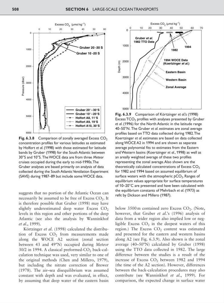
suggests that no portion of the Atlantic Ocean can
necessarily be assumed to be free of Excess CO 2 . It
is therefore possible that Gruber (1998) may have
slightly underestimated deep water Excess CO 2
levels in this region and other portions of the deep
Atlantic (see also the analysis by Wanninkhof
et al., 1999).
Körtzinger et al. (1998) calculated the distribution of Excess CO 2 from measurements made
along the WOCE A2 section (zonal section
between 43 and 49°N) occupied during Meteor
30/2 in 1994. A classical preformed-CO 2 back-calculation technique was used, very similar to one of
the original methods (Chen and Millero, 1979),
but including the nitrate correction of Brewer
(1978). The air–sea disequilibrium was assumed
constant with depth and was evaluated, in effect,
by assuming that deep water of the eastern basin
below 3500 m contained zero Excess CO 2 . (Note,
however, that Gruber et al.’s (1996) analysis of
data from a wider region also implied low or negligible Excess CO 2 in the deepest waters of this
region.) The Excess CO 2 content was estimated
and presented for the eastern and western basins
along A2 (see Fig. 6.3.9). Also shown is the zonal
average (40–50°N) calculated by Gruber (1998)
using the TTO data collected in 1982. The large
difference between the studies is a result of the
increase of Excess CO 2 between 1982 and 1994
(the time of the A2 section). However, differences
between the back-calculation procedures may also
contribute (see Wanninkhof et al., 1999). For
comparison, the expected change in surface water
SECTION 6 LARGE-SCALE OCEAN TRANSPORTS
508
Excess CO 2 (μmol kg
–1 )
Depth (m)
0
1000
2000
3000
4000
5000
Gruber et al.
1982 TTO Data
1994 WOCE Data
(Koertzinger et al.)
Eastern Basin
Western Basin
Zonal Average
1982
1994
0
1 0
2 0
3 0
4 0
5 0
6 0
7 0
Fig. 6.3.9 Comparison of Körtzinger et al.’s (1998)
Excess TCO 2 profiles with analyses presented by Gruber
et al. (1996) for the North Atlantic in the latitude range
40–50°N. The Gruber et al. estimates are zonal average
profiles based on TTO data collected during 1982.The
Koertzinger et al. estimates are based on data collected
along WOCE A2 in 1994 and are shown as separate
average polynomial fits to estimates from the Eastern
and Western basins (Koertzinger et al., 1998) as well as
an areally weighted average of these two profiles
representing the zonal average.Also shown are the
theoretically calculated concentrations of Excess CO 2
for 1982 and 1994 based on assumed equilibrium of
surface waters with the atmospheric pCO 2 . Ranges of
equilibrium values appropriate for surface temperatures
of 10–20°C are presented and have been calculated with
the equilibrium constants of Mehrbach et al. (1973) as
refit by Dickson and Millero (1987).
Excess CO 2 (μmol kg
–1
)
Pressure (dbar)
0
2000
1000
3000
4000
5000
6000
Gruber 20°–30°S
Gruber 10°–20°S
Holfort A8, 11°S
Holfort A9, 19°S
Holfort A10, 30°S
Gruber 20 -30 S
Gruber 10 -20 S
0
1 0
2 0
3 0
4 0
5 0
6 0
Fig. 6.3.8 Comparison of zonally averaged Excess CO 2
concentration profiles for various latitudes as estimated
by Holfort et al. (1998) with those estimated for latitude
bands by Gruber (1998) for the South Atlantic between
30°S and 10°S. The WOCE data are from three Meteor
cruises occupied during the early to mid-1990s.The
Gruber analyses are based primarily on analysis of data
collected during the South Atlantic Ventilation Experiment
(SAVE) during 1987–89 but include some WOCE data.
necessarily be assumed to be free of Excess CO 2 . It
is therefore possible that Gruber (1998) may have
slightly underestimated deep water Excess CO 2
levels in this region and other portions of the deep
Atlantic (see also the analysis by Wanninkhof
et al., 1999).
Körtzinger et al. (1998) calculated the distribution of Excess CO 2 from measurements made
along the WOCE A2 section (zonal section
between 43 and 49°N) occupied during Meteor
30/2 in 1994. A classical preformed-CO 2 back-calculation technique was used, very similar to one of
the original methods (Chen and Millero, 1979),
but including the nitrate correction of Brewer
(1978). The air–sea disequilibrium was assumed
constant with depth and was evaluated, in effect,
by assuming that deep water of the eastern basin
below 3500 m contained zero Excess CO 2 . (Note,
however, that Gruber et al.’s (1996) analysis of
data from a wider region also implied low or negligible Excess CO 2 in the deepest waters of this
region.) The Excess CO 2 content was estimated
and presented for the eastern and western basins
along A2 (see Fig. 6.3.9). Also shown is the zonal
average (40–50°N) calculated by Gruber (1998)
using the TTO data collected in 1982. The large
difference between the studies is a result of the
increase of Excess CO 2 between 1982 and 1994
(the time of the A2 section). However, differences
between the back-calculation procedures may also
contribute (see Wanninkhof et al., 1999). For
comparison, the expected change in surface water
SECTION 6 LARGE-SCALE OCEAN TRANSPORTS
508
Excess CO 2 (μmol kg
–1 )
Depth (m)
0
1000
2000
3000
4000
5000
Gruber et al.
1982 TTO Data
1994 WOCE Data
(Koertzinger et al.)
Eastern Basin
Western Basin
Zonal Average
1982
1994
0
1 0
2 0
3 0
4 0
5 0
6 0
7 0
Fig. 6.3.9 Comparison of Körtzinger et al.’s (1998)
Excess TCO 2 profiles with analyses presented by Gruber
et al. (1996) for the North Atlantic in the latitude range
40–50°N. The Gruber et al. estimates are zonal average
profiles based on TTO data collected during 1982.The
Koertzinger et al. estimates are based on data collected
along WOCE A2 in 1994 and are shown as separate
average polynomial fits to estimates from the Eastern
and Western basins (Koertzinger et al., 1998) as well as
an areally weighted average of these two profiles
representing the zonal average.Also shown are the
theoretically calculated concentrations of Excess CO 2
for 1982 and 1994 based on assumed equilibrium of
surface waters with the atmospheric pCO 2 . Ranges of
equilibrium values appropriate for surface temperatures
of 10–20°C are presented and have been calculated with
the equilibrium constants of Mehrbach et al. (1973) as
refit by Dickson and Millero (1987).
Excess CO 2 (μmol kg
–1
)
Pressure (dbar)
0
2000
1000
3000
4000
5000
6000
Gruber 20°–30°S
Gruber 10°–20°S
Holfort A8, 11°S
Holfort A9, 19°S
Holfort A10, 30°S
Gruber 20 -30 S
Gruber 10 -20 S
0
1 0
2 0
3 0
4 0
5 0
6 0
Fig. 6.3.8 Comparison of zonally averaged Excess CO 2
concentration profiles for various latitudes as estimated
by Holfort et al. (1998) with those estimated for latitude
bands by Gruber (1998) for the South Atlantic between
30°S and 10°S. The WOCE data are from three Meteor
cruises occupied during the early to mid-1990s.The
Gruber analyses are based primarily on analysis of data
collected during the South Atlantic Ventilation Experiment
(SAVE) during 1987–89 but include some WOCE data.