

1985b). Gruber et al. (1996) clarified and partially
addressed some of the problematic issues inherent
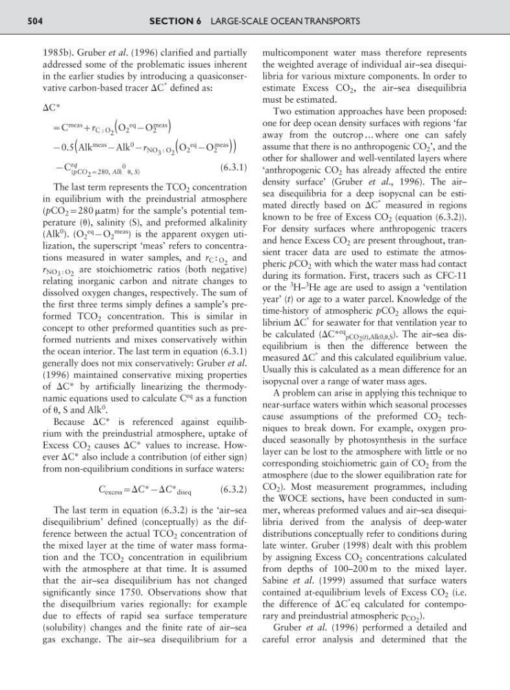
in the earlier studies by introducing a quasiconservative carbon-based tracer ⌬C
* defined as:
⌬C*
:C
meas
;r C : O 2 (O 2
eq
9O 2
meas
)
90.5(Alk
meas
9Alk
0
9r NO 3 : O 2 (O 2
eq
9O 2
meas
))
9C
eq
(pCO 2 :280, Alk
0 , S)
(6.3.1)
The last term represents the TCO 2 concentration
in equilibrium with the preindustrial atmosphere
(pCO 2 :280 atm) for the sample’s potential temperature (), salinity (S), and preformed alkalinity
(Alk
0
). (O 2
eq
9O 2
meas
) is the apparent oxygen utilization, the superscript ‘meas’ refers to concentrations measured in water samples, and r C : O 2 and
r NO 3 : O 2 are stoichiometric ratios (both negative)
relating inorganic carbon and nitrate changes to
dissolved oxygen changes, respectively. The sum of
the first three terms simply defines a sample’s preformed TCO 2 concentration. This is similar in
concept to other preformed quantities such as preformed nutrients and mixes conservatively within
the ocean interior. The last term in equation (6.3.1)
generally does not mix conservatively: Gruber et al.
(1996) maintained conservative mixing properties
of ⌬C* by artificially linearizing the thermodynamic equations used to calculate C
eq as a function
of , S and Alk
0
.
Because ⌬C* is referenced against equilibrium with the preindustrial atmosphere, uptake of
Excess CO 2 causes ⌬C* values to increase. However ⌬C* also include a contribution (of either sign)
from non-equilibrium conditions in surface waters:
C excess :⌬C*9⌬C* diseq
(6.3.2)
The last term in equation (6.3.2) is the ‘air–sea
disequilibrium’ defined (conceptually) as the difference between the actual TCO 2 concentration of
the mixed layer at the time of water mass formation and the TCO 2 concentration in equilibrium
with the atmosphere at that time. It is assumed
that the air–sea disequilibrium has not changed
significantly since 1750. Observations show that
the disequilbrium varies regionally: for example
due to effects of rapid sea surface temperature
(solubility) changes and the finite rate of air–sea
gas exchange. The air–sea disequilibrium for a
multicomponent water mass therefore represents
the weighted average of individual air–sea disequilibria for various mixture components. In order to
estimate Excess CO 2 , the air–sea disequilibria
must be estimated.
Two estimation approaches have been proposed:
one for deep ocean density surfaces with regions ‘far
away from the outcrop … where one can safely
assume that there is no anthropogenic CO 2 ’, and the
other for shallower and well-ventilated layers where
‘anthropogenic CO 2 has already affected the entire
density surface’ (Gruber et al., 1996). The air–
sea disequilibria for a deep isopycnal can be estimated directly based on ⌬C
* measured in regions
known to be free of Excess CO 2 (equation (6.3.2)).
For density surfaces where anthropogenic tracers
and hence Excess CO 2 are present throughout, transient tracer data are used to estimate the atmospheric pCO 2 with which the water mass had contact
during its formation. First, tracers such as CFC-11
or the
3
H–
3
He age are used to assign a ‘ventilation
year’ (t) or age to a water parcel. Knowledge of the
time-history of atmospheric pCO 2 allows the equilibrium ⌬C
* for seawater for that ventilation year to
be calculated (⌬C*
eq
pCO 2 (t),Alk0,,S ). The air–sea disequilibrium is then the difference between the
measured ⌬C
* and this calculated equilibrium value.
Usually this is calculated as a mean difference for an
isopycnal over a range of water mass ages.
A problem can arise in applying this technique to
near-surface waters within which seasonal processes
cause assumptions of the preformed CO 2 techniques to break down. For example, oxygen produced seasonally by photosynthesis in the surface
layer can be lost to the atmosphere with little or no
corresponding stoichiometric gain of CO 2 from the
atmosphere (due to the slower equilibration rate for
CO 2 ). Most measurement programmes, including
the WOCE sections, have been conducted in summer, whereas preformed values and air–sea disequilibria derived from the analysis of deep-water
distributions conceptually refer to conditions during
late winter. Gruber (1998) dealt with this problem
by assigning Excess CO 2 concentrations calculated
from depths of 100–200 m to the mixed layer.
Sabine et al. (1999) assumed that surface waters
contained at-equilibrium levels of Excess CO 2 (i.e.
the difference of ⌬C
*
eq calculated for contemporary and preindustrial atmospheric p CO 2 ).
Gruber et al. (1996) performed a detailed and
careful error analysis and determined that the
SECTION 6 LARGE-SCALE OCEAN TRANSPORTS
504
addressed some of the problematic issues inherent
in the earlier studies by introducing a quasiconservative carbon-based tracer ⌬C
* defined as:
⌬C*
:C
meas
;r C : O 2 (O 2
eq
9O 2
meas
)
90.5(Alk
meas
9Alk
0
9r NO 3 : O 2 (O 2
eq
9O 2
meas
))
9C
eq
(pCO 2 :280, Alk
0 , S)
(6.3.1)
The last term represents the TCO 2 concentration
in equilibrium with the preindustrial atmosphere
(pCO 2 :280 atm) for the sample’s potential temperature (), salinity (S), and preformed alkalinity
(Alk
0
). (O 2
eq
9O 2
meas
) is the apparent oxygen utilization, the superscript ‘meas’ refers to concentrations measured in water samples, and r C : O 2 and
r NO 3 : O 2 are stoichiometric ratios (both negative)
relating inorganic carbon and nitrate changes to
dissolved oxygen changes, respectively. The sum of
the first three terms simply defines a sample’s preformed TCO 2 concentration. This is similar in
concept to other preformed quantities such as preformed nutrients and mixes conservatively within
the ocean interior. The last term in equation (6.3.1)
generally does not mix conservatively: Gruber et al.
(1996) maintained conservative mixing properties
of ⌬C* by artificially linearizing the thermodynamic equations used to calculate C
eq as a function
of , S and Alk
0
.
Because ⌬C* is referenced against equilibrium with the preindustrial atmosphere, uptake of
Excess CO 2 causes ⌬C* values to increase. However ⌬C* also include a contribution (of either sign)
from non-equilibrium conditions in surface waters:
C excess :⌬C*9⌬C* diseq
(6.3.2)
The last term in equation (6.3.2) is the ‘air–sea
disequilibrium’ defined (conceptually) as the difference between the actual TCO 2 concentration of
the mixed layer at the time of water mass formation and the TCO 2 concentration in equilibrium
with the atmosphere at that time. It is assumed
that the air–sea disequilibrium has not changed
significantly since 1750. Observations show that
the disequilbrium varies regionally: for example
due to effects of rapid sea surface temperature
(solubility) changes and the finite rate of air–sea
gas exchange. The air–sea disequilibrium for a
multicomponent water mass therefore represents
the weighted average of individual air–sea disequilibria for various mixture components. In order to
estimate Excess CO 2 , the air–sea disequilibria
must be estimated.
Two estimation approaches have been proposed:
one for deep ocean density surfaces with regions ‘far
away from the outcrop … where one can safely
assume that there is no anthropogenic CO 2 ’, and the
other for shallower and well-ventilated layers where
‘anthropogenic CO 2 has already affected the entire
density surface’ (Gruber et al., 1996). The air–
sea disequilibria for a deep isopycnal can be estimated directly based on ⌬C
* measured in regions
known to be free of Excess CO 2 (equation (6.3.2)).
For density surfaces where anthropogenic tracers
and hence Excess CO 2 are present throughout, transient tracer data are used to estimate the atmospheric pCO 2 with which the water mass had contact
during its formation. First, tracers such as CFC-11
or the
3
H–
3
He age are used to assign a ‘ventilation
year’ (t) or age to a water parcel. Knowledge of the
time-history of atmospheric pCO 2 allows the equilibrium ⌬C
* for seawater for that ventilation year to
be calculated (⌬C*
eq
pCO 2 (t),Alk0,,S ). The air–sea disequilibrium is then the difference between the
measured ⌬C
* and this calculated equilibrium value.
Usually this is calculated as a mean difference for an
isopycnal over a range of water mass ages.
A problem can arise in applying this technique to
near-surface waters within which seasonal processes
cause assumptions of the preformed CO 2 techniques to break down. For example, oxygen produced seasonally by photosynthesis in the surface
layer can be lost to the atmosphere with little or no
corresponding stoichiometric gain of CO 2 from the
atmosphere (due to the slower equilibration rate for
CO 2 ). Most measurement programmes, including
the WOCE sections, have been conducted in summer, whereas preformed values and air–sea disequilibria derived from the analysis of deep-water
distributions conceptually refer to conditions during
late winter. Gruber (1998) dealt with this problem
by assigning Excess CO 2 concentrations calculated
from depths of 100–200 m to the mixed layer.
Sabine et al. (1999) assumed that surface waters
contained at-equilibrium levels of Excess CO 2 (i.e.
the difference of ⌬C
*
eq calculated for contemporary and preindustrial atmospheric p CO 2 ).
Gruber et al. (1996) performed a detailed and
careful error analysis and determined that the
SECTION 6 LARGE-SCALE OCEAN TRANSPORTS
504