

The carbon cycle GCMs can also be used to
assess the regional distribution of the uptake of
Excess CO 2 from the atmosphere. This uptake is
referred to by modellers as the ‘Perturbation Flux’,
which is the perturbation of the natural air–sea
CO 2 flux associated with higher concentrations of
atmospheric CO 2 . The issue of where Excess CO 2
is taken up across the air–sea interface may be of
critical importance for our ability to predict future
CO 2 uptake by the oceans under a climate-altered
ocean circulation (Caldeira and Duffy, 2000). As
noted earlier (Section 6.3.2.1), the uptake of Excess
CO 2 cannot be determined from air–sea flux estimates and hence model predictions of the geographical distribution of this flux cannot readily be
evaluated. Model predictions of the total (natural
plus Excess) flux can, of course, be compared
against the observation-based estimates. Within
this chapter I argue that use of CO 2 survey data to
estimate budgets for the transport and storage of
Excess CO 2 offers a way to separate these components on regional scales (Section 6.3.4.3).
Global inverse modelling of atmospheric CO 2
The carbon storage term for the terrestrial biosphere is notoriously difficult to assess directly and
has been assessed perhaps most reliably through
consideration of the global mass balance for the
other reservoirs (atmosphere and ocean), leaving
the terrestrial biosphere storage term to be calculated by difference. Most recently atmospheric
O 2 /N 2 time series have proven particularly useful
for this. Information concerning the specific location and mechanisms of carbon storage in the terrestrial biosphere has proven particularly difficult
to obtain. Over the past decade attention has
focused on inferring net fluxes of carbon into
and out of the terrestrial biosphere based on
inverse modelling of atmospheric CO 2 data. This
approach utilizes spatially resolved data on fossil
fuel CO 2 release and atmospheric concentrations
as constraints within atmospheric transport models. The task is to find a distribution of carbon
sources and sinks that, when combined with
known fossil fuel sources, reproduces the observed
spatial distributions of CO 2 (or its stable isotopes)
in the atmosphere.
Most examples of this approach have focussed
on modelling meridional CO 2 gradients in the
atmosphere (e.g. studies by Keeling and Heimann,
1986; Keeling et al., 1989; Tans et al., 1990;
Ciais et al., 1995; etc.). The natural preindustrial
transport of carbon between the hemispheres is,
however, a key factor for the interpretation of
present-day meridional gradients. This is illustrated schematically in Figure 6.3.2. Early studies
6.3 Storage and Transport of Excess CO 2 in the Oceans
493
Wallace
Specific inventory (mol C m
–2
)
0
0˚
20
20˚
40
40˚
60
60˚
80
80˚N
100
Preformed CO
2
GCM
2.5D model
Total inventories
Observations:
GCM simulation: 18.4 PgC
2.5D model:
18.7 PgC
20.0 PgC
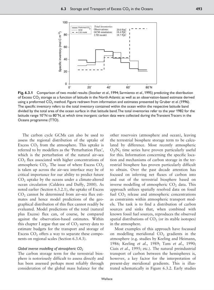
Fig. 6.3.1 Comparison of two model results (Stocker et al., 1994; Sarmiento et al., 1995) predicting the distribution
of Excess CO 2 storage as a function of latitude in the North Atlantic as well as an observation-based estimate derived
using a preformed CO 2 method. Figure redrawn from information and estimates presented by Gruber et al. (1996).
The specific inventory refers to the total inventory contained within the ocean within the respective latitude band
divided by the total area of the ocean surface in that latitude band.The total inventories refer to the year 1982 for the
latitude range 10°N to 80°N, at which time inorganic carbon data were collected during the Transient Tracers in the
Oceans programme (TTO).
assess the regional distribution of the uptake of
Excess CO 2 from the atmosphere. This uptake is
referred to by modellers as the ‘Perturbation Flux’,
which is the perturbation of the natural air–sea
CO 2 flux associated with higher concentrations of
atmospheric CO 2 . The issue of where Excess CO 2
is taken up across the air–sea interface may be of
critical importance for our ability to predict future
CO 2 uptake by the oceans under a climate-altered
ocean circulation (Caldeira and Duffy, 2000). As
noted earlier (Section 6.3.2.1), the uptake of Excess
CO 2 cannot be determined from air–sea flux estimates and hence model predictions of the geographical distribution of this flux cannot readily be
evaluated. Model predictions of the total (natural
plus Excess) flux can, of course, be compared
against the observation-based estimates. Within
this chapter I argue that use of CO 2 survey data to
estimate budgets for the transport and storage of
Excess CO 2 offers a way to separate these components on regional scales (Section 6.3.4.3).
Global inverse modelling of atmospheric CO 2
The carbon storage term for the terrestrial biosphere is notoriously difficult to assess directly and
has been assessed perhaps most reliably through
consideration of the global mass balance for the
other reservoirs (atmosphere and ocean), leaving
the terrestrial biosphere storage term to be calculated by difference. Most recently atmospheric
O 2 /N 2 time series have proven particularly useful
for this. Information concerning the specific location and mechanisms of carbon storage in the terrestrial biosphere has proven particularly difficult
to obtain. Over the past decade attention has
focused on inferring net fluxes of carbon into
and out of the terrestrial biosphere based on
inverse modelling of atmospheric CO 2 data. This
approach utilizes spatially resolved data on fossil
fuel CO 2 release and atmospheric concentrations
as constraints within atmospheric transport models. The task is to find a distribution of carbon
sources and sinks that, when combined with
known fossil fuel sources, reproduces the observed
spatial distributions of CO 2 (or its stable isotopes)
in the atmosphere.
Most examples of this approach have focussed
on modelling meridional CO 2 gradients in the
atmosphere (e.g. studies by Keeling and Heimann,
1986; Keeling et al., 1989; Tans et al., 1990;
Ciais et al., 1995; etc.). The natural preindustrial
transport of carbon between the hemispheres is,
however, a key factor for the interpretation of
present-day meridional gradients. This is illustrated schematically in Figure 6.3.2. Early studies
6.3 Storage and Transport of Excess CO 2 in the Oceans
493
Wallace
Specific inventory (mol C m
–2
)
0
0˚
20
20˚
40
40˚
60
60˚
80
80˚N
100
Preformed CO
2
GCM
2.5D model
Total inventories
Observations:
GCM simulation: 18.4 PgC
2.5D model:
18.7 PgC
20.0 PgC
Fig. 6.3.1 Comparison of two model results (Stocker et al., 1994; Sarmiento et al., 1995) predicting the distribution
of Excess CO 2 storage as a function of latitude in the North Atlantic as well as an observation-based estimate derived
using a preformed CO 2 method. Figure redrawn from information and estimates presented by Gruber et al. (1996).
The specific inventory refers to the total inventory contained within the ocean within the respective latitude band
divided by the total area of the ocean surface in that latitude band.The total inventories refer to the year 1982 for the
latitude range 10°N to 80°N, at which time inorganic carbon data were collected during the Transient Tracers in the
Oceans programme (TTO).