

sections covering all ocean basins taken prior to the
WOCE observational period. In a sense, it is one
summary of the global ocean circulation and of
ocean heat transport prior to WOCE. Here we display their pattern for the deep circulation colder
than 3.5°C (Fig. 6.1.7, see Plate 6.1.7, p. 492) and
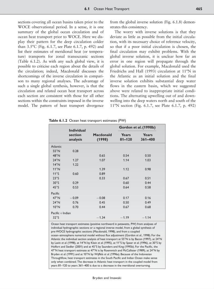
list their estimates of meridional heat (or temperature) transports for zonal transoceanic sections
(Table 6.1.2). As with any such global view, it is
possible to criticise each region about the details of
the circulation; indeed, Macdonald discusses the
shortcomings of the inverse circulation in comparison to many regional analyses. The advantage of
such a single global synthesis, however, is that the
circulation and related ocean heat transport across
each section are consistent with those for all other
sections within the constraints imposed in the inverse
model. The pattern of heat transport divergence
from the global inverse solution (Fig. 6.1.8) demonstrates this consistency.
The worry with inverse solutions is that they
deviate as little as possible from the initial circulation, with its necessary choice of reference velocity,
so that if a poor initial circulation is chosen, the
final circulation may exhibit problems. With the
global inverse solution, it is unclear how far an
error in one region will propagate through the
global solution. For example, Macdonald used the
Friedrichs and Hall (1993) circulation at 11°N in
the Atlantic as an initial solution and the final
inverse solution exhibits substantial deep water
flows in the eastern basin, which we suggested
above were related to inappropriate initial conditions. The alternating upwelling out of and downwelling into the deep waters north and south of the
11°N section (Fig. 6.1.7, see Plate 6.1.7, p. 492)
6.1 Ocean Heat Transport
465
Bryden and Imawaki
Table 6.1.2 Ocean heat transport estimates (PW)
Individual
Gordon et al. (1998b)
section
Macdonald
Years
Years
analysis
(1998)
81–120
361–400
Atlantic
55°N
0.28
48°N
0.65
0.54
0.50
24°N
1.27
1.07
1.14
1.03
14°N
1.22
11°N
1.39
1.12
0.98
11°S
0.60
0.89
23°S
0.33
0.67
0.51
30°S
0.29
0.60
0.44
45°S
0.53
0.64
0.58
Pacific
47°N
90.09
90.08
0.17
0.16
24°N
0.76
0.45
0.50
0.49
10°N
0.70
0.44
0.67
0.68
Pacific;Indian
32°S
91.34
91.19
91.14
Ocean heat transport estimates (positive northward in petawatts, PW) from analyses of
individual hydrographic sections or a regional inverse model, from a global synthesis of
pre-WOCE hydrographic sections (Macdonald, 1998), and from a coupled
ocean–atmosphere numerical model without flux adjustment (Gordon et al., 1998). For the
Atlantic the individual section analysis of heat transport at 55°N is by Bacon (1997), at 24°N
by Lavín et al. (1998), at 14°N by Klein et al. (1995), at 11°S by Speer et al. (1996), at 30°S by
Holfort and Siedler (2001) and at 45°S by Saunders and King (1995b). For the Pacific, the
47°N heat transport estimate at 47°N is by Roemmich and McCallister (1989), at 24°N by
Bryden et al. (1991) and at 10°N by Wijffels et al. (1996a). Because of the Indonesian
Throughflow, heat transport estimates in the South Pacific and Indian Ocean make sense
only when combined. The decrease in Atlantic heat transport in the coupled model from
years 81–120 to years 361–400 is due to a decrease in the meridional overturning.
WOCE observational period. In a sense, it is one
summary of the global ocean circulation and of
ocean heat transport prior to WOCE. Here we display their pattern for the deep circulation colder
than 3.5°C (Fig. 6.1.7, see Plate 6.1.7, p. 492) and
list their estimates of meridional heat (or temperature) transports for zonal transoceanic sections
(Table 6.1.2). As with any such global view, it is
possible to criticise each region about the details of
the circulation; indeed, Macdonald discusses the
shortcomings of the inverse circulation in comparison to many regional analyses. The advantage of
such a single global synthesis, however, is that the
circulation and related ocean heat transport across
each section are consistent with those for all other
sections within the constraints imposed in the inverse
model. The pattern of heat transport divergence
from the global inverse solution (Fig. 6.1.8) demonstrates this consistency.
The worry with inverse solutions is that they
deviate as little as possible from the initial circulation, with its necessary choice of reference velocity,
so that if a poor initial circulation is chosen, the
final circulation may exhibit problems. With the
global inverse solution, it is unclear how far an
error in one region will propagate through the
global solution. For example, Macdonald used the
Friedrichs and Hall (1993) circulation at 11°N in
the Atlantic as an initial solution and the final
inverse solution exhibits substantial deep water
flows in the eastern basin, which we suggested
above were related to inappropriate initial conditions. The alternating upwelling out of and downwelling into the deep waters north and south of the
11°N section (Fig. 6.1.7, see Plate 6.1.7, p. 492)
6.1 Ocean Heat Transport
465
Bryden and Imawaki
Table 6.1.2 Ocean heat transport estimates (PW)
Individual
Gordon et al. (1998b)
section
Macdonald
Years
Years
analysis
(1998)
81–120
361–400
Atlantic
55°N
0.28
48°N
0.65
0.54
0.50
24°N
1.27
1.07
1.14
1.03
14°N
1.22
11°N
1.39
1.12
0.98
11°S
0.60
0.89
23°S
0.33
0.67
0.51
30°S
0.29
0.60
0.44
45°S
0.53
0.64
0.58
Pacific
47°N
90.09
90.08
0.17
0.16
24°N
0.76
0.45
0.50
0.49
10°N
0.70
0.44
0.67
0.68
Pacific;Indian
32°S
91.34
91.19
91.14
Ocean heat transport estimates (positive northward in petawatts, PW) from analyses of
individual hydrographic sections or a regional inverse model, from a global synthesis of
pre-WOCE hydrographic sections (Macdonald, 1998), and from a coupled
ocean–atmosphere numerical model without flux adjustment (Gordon et al., 1998). For the
Atlantic the individual section analysis of heat transport at 55°N is by Bacon (1997), at 24°N
by Lavín et al. (1998), at 14°N by Klein et al. (1995), at 11°S by Speer et al. (1996), at 30°S by
Holfort and Siedler (2001) and at 45°S by Saunders and King (1995b). For the Pacific, the
47°N heat transport estimate at 47°N is by Roemmich and McCallister (1989), at 24°N by
Bryden et al. (1991) and at 10°N by Wijffels et al. (1996a). Because of the Indonesian
Throughflow, heat transport estimates in the South Pacific and Indian Ocean make sense
only when combined. The decrease in Atlantic heat transport in the coupled model from
years 81–120 to years 361–400 is due to a decrease in the meridional overturning.