

the observations at Station 66 the required buoyancy loss is found by calculating
g/ 0 ͐⌬ dz
where g (10 m s
92
) is the acceleration due to gravity,
0 (Ϸ1034 kg m
93
) is the reference density, z is the
depth and ⌬ is the difference in density between
Station 66 and a density of 1034.694 kg m
93
. This
yields a buoyancy loss of 0.47 m
2 s
92
, which can be
converted to joules by dividing by g␣/ 0 c where g
and 0 are as before, ␣ (10
94 °C
91
) is the thermal
expansion of water and c (4.2 kJ kg
91 °C
91
) is the
specific heat capacity of seawater. The conversion suggests a heat loss of Ϸ210
9 J m
92 will
create a mixed layer to 2000 m and density of
1034.694 kg m
93
. Since Station 66 was obtained on
25 February, only 35 days before the usual end of
the cooling season on 1 April, it would require a
heat flux of about 630 W m
92 over the 35 days.
Although such high heat fluxes have been observed
in the area (see The Lab Sea Group, 1998), they are
relatively rare and only sustained for significant
periods in exceptionally severe winters.
A similar buoyancy calculation starting with
data obtained near the end of summer in 1996
yields Ϸ410
9 J m
92 as the heat loss required
to create a convection layer to 2000 m or
1034.694 kg m
93
. Over the approximately 180
days of cooling between 1 October and 1 April this
would require an average heat flux of
Ϸ250 W m
92
. Smith and Dobson (1984) calculated
that between October and April the average heat
loss from the central Labrador Sea, based on meteorological observations at Ocean Weather Ship
Bravo (56.5°N 51°W) between 1946 and 1974, is
Ϸ150<60 W m
92
. These values imply that a winter
severe enough to produce convection to 2000 m, i.e.
Ϸ250 W m
92 for 180 days, would occur when the
heat loss over the winter was larger than the average by Ϸ1.5 standard deviations or roughly once in
10 years; this is about what is observed.
The buoyancy calculation is also useful because
it is dependent only on the density profile. If the
density profile remains unchanged, the heat loss
required to produce a mixed layer to a given depth
remains the same; independent of changes in the
temperature and salinity profiles. In the Labrador
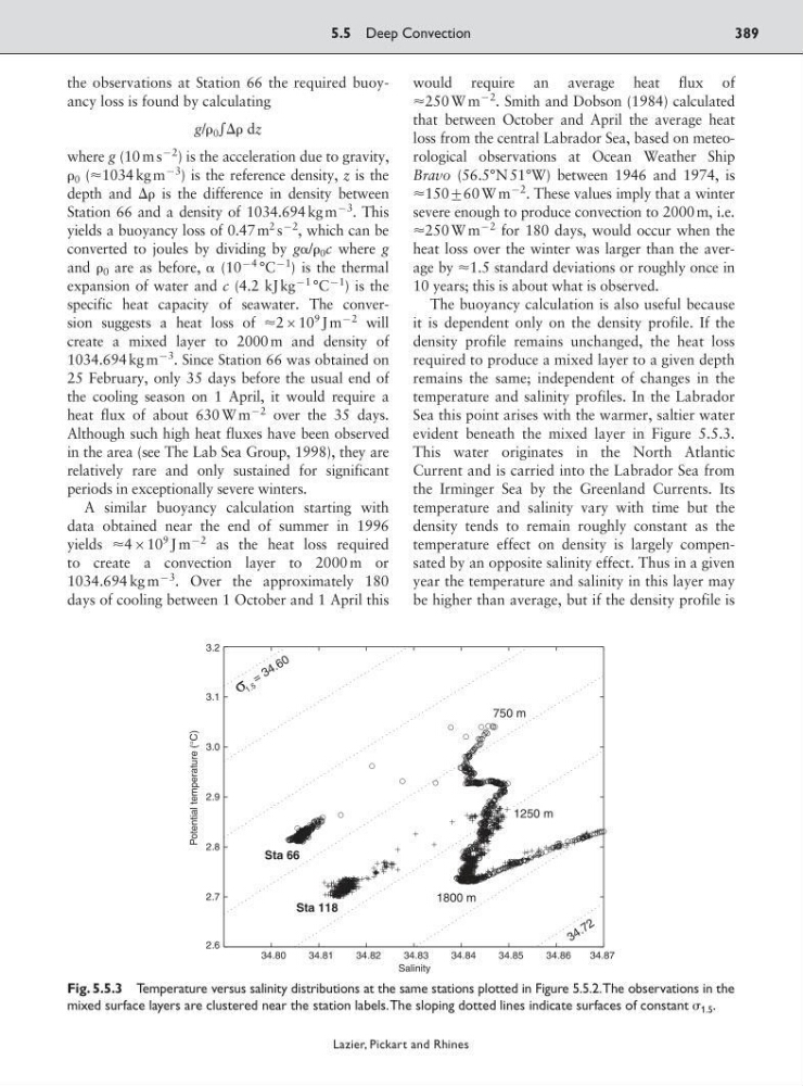
Sea this point arises with the warmer, saltier water
evident beneath the mixed layer in Figure 5.5.3.
This water originates in the North Atlantic
Current and is carried into the Labrador Sea from
the Irminger Sea by the Greenland Currents. Its
temperature and salinity vary with time but the
density tends to remain roughly constant as the
temperature effect on density is largely compensated by an opposite salinity effect. Thus in a given
year the temperature and salinity in this layer may
be higher than average, but if the density profile is
5.5 Deep Convection
389
Lazier, Pickart and Rhines
34.80
34.81
34.82
34.83
34.84
34.85
34.86
34.87
2.6
2.7
2.8
2.9
3.0
3.1
3.2
Salinity
1 .5
σ
= 3 4 . 6 0
3 4 . 7 2
Sta 66
Sta 118
750 m
1250 m
1800 m
Potential temperature (°C)
Fig. 5.5.3 Temperature versus salinity distributions at the same stations plotted in Figure 5.5.2.The observations in the
mixed surface layers are clustered near the station labels.The sloping dotted lines indicate surfaces of constant 1.5 .
g/ 0 ͐⌬ dz
where g (10 m s
92
) is the acceleration due to gravity,
0 (Ϸ1034 kg m
93
) is the reference density, z is the
depth and ⌬ is the difference in density between
Station 66 and a density of 1034.694 kg m
93
. This
yields a buoyancy loss of 0.47 m
2 s
92
, which can be
converted to joules by dividing by g␣/ 0 c where g
and 0 are as before, ␣ (10
94 °C
91
) is the thermal
expansion of water and c (4.2 kJ kg
91 °C
91
) is the
specific heat capacity of seawater. The conversion suggests a heat loss of Ϸ210
9 J m
92 will
create a mixed layer to 2000 m and density of
1034.694 kg m
93
. Since Station 66 was obtained on
25 February, only 35 days before the usual end of
the cooling season on 1 April, it would require a
heat flux of about 630 W m
92 over the 35 days.
Although such high heat fluxes have been observed
in the area (see The Lab Sea Group, 1998), they are
relatively rare and only sustained for significant
periods in exceptionally severe winters.
A similar buoyancy calculation starting with
data obtained near the end of summer in 1996
yields Ϸ410
9 J m
92 as the heat loss required
to create a convection layer to 2000 m or
1034.694 kg m
93
. Over the approximately 180
days of cooling between 1 October and 1 April this
would require an average heat flux of
Ϸ250 W m
92
. Smith and Dobson (1984) calculated
that between October and April the average heat
loss from the central Labrador Sea, based on meteorological observations at Ocean Weather Ship
Bravo (56.5°N 51°W) between 1946 and 1974, is
Ϸ150<60 W m
92
. These values imply that a winter
severe enough to produce convection to 2000 m, i.e.
Ϸ250 W m
92 for 180 days, would occur when the
heat loss over the winter was larger than the average by Ϸ1.5 standard deviations or roughly once in
10 years; this is about what is observed.
The buoyancy calculation is also useful because
it is dependent only on the density profile. If the
density profile remains unchanged, the heat loss
required to produce a mixed layer to a given depth
remains the same; independent of changes in the
temperature and salinity profiles. In the Labrador
Sea this point arises with the warmer, saltier water
evident beneath the mixed layer in Figure 5.5.3.
This water originates in the North Atlantic
Current and is carried into the Labrador Sea from
the Irminger Sea by the Greenland Currents. Its
temperature and salinity vary with time but the
density tends to remain roughly constant as the
temperature effect on density is largely compensated by an opposite salinity effect. Thus in a given
year the temperature and salinity in this layer may
be higher than average, but if the density profile is
5.5 Deep Convection
389
Lazier, Pickart and Rhines
34.80
34.81
34.82
34.83
34.84
34.85
34.86
34.87
2.6
2.7
2.8
2.9
3.0
3.1
3.2
Salinity
1 .5
σ
= 3 4 . 6 0
3 4 . 7 2
Sta 66
Sta 118
750 m
1250 m
1800 m
Potential temperature (°C)
Fig. 5.5.3 Temperature versus salinity distributions at the same stations plotted in Figure 5.5.2.The observations in the
mixed surface layers are clustered near the station labels.The sloping dotted lines indicate surfaces of constant 1.5 .