

that atmospheric forcing (and mixing) is confined
to within a relatively thin surface layer of the ocean,
and vanishes in the stratified water below.
One of the first successful attempts to estimate the three-dimensional mass flux through the
thermocline was by Montgomery (1938), who
constructed a streamtube model whose lateral
boundaries were observed isohalines, and whose
upper and lower boundaries were observed density
surfaces. This streamtube had an open mouth at
the base of the upper ocean Ekman layer, and then
followed a path defined by the observed salinity
and density fields downward and equatorward
into the North Atlantic main thermocline. The
mass flux through such a streamtube was found
to be roughly consistent with the convergence of
the Ekman transport over the streamtube mouth.
Montgomery’s streamtube model was regional in
scope and diagnostic in that it required detailed
information on the distribution of the tracers
(salinity and density) that are themselves the result
of the circulation. Though far from a complete
model, Montgomery’s streamtube analysis was
nevertheless a crucial step in establishing a quantitative connection between wind forcing, tracer
fields and the three-dimensional circulation.
Another, and crucial, connection between the
thermocline circulation and the wind fields is given
by the Sverdrup theory that relates the vertical
integral of the meridional current (sea surface to
seafloor) directly to the wind stress curl. The
Sverdrup relation makes no distinction between
the directly wind-driven surface layer and the
geostrophic (unforced) flow below. The seminal circulation model of Luyten, Pedlosky and Stommel
(1983, hereafter, LPS) might be viewed as a model
that makes explicit the distinction between the
ocean surface layer, which is in direct contact with
the atmosphere and thus subject to a stress curl,
and the nearly unforced (or adiabatic) thermocline
below. The Sverdrup relation for transport was
assumed to hold within the thermocline alone,
and the thermocline water (represented by a few
discrete layers) was assumed to be in contact with
the atmosphere at appropriate, specified latitudes.
The result was a three-dimensional circulation and
thermocline structure that gave remarkable insight
into major features of the subtropical thermocline.
In particular, the LPS model showed that the thermocline circulation could be envisioned as made
up of domains having quite distinct dynamics and
characteristic paths through the thermocline by
SECTION 5 FORMATION AND TRANSPORT OF WATER MASSES
358
Temperature (°C)
Temperature (°C)
Salinity (ppt)
Salinity (ppt)
(a)
(b)
.8 35.0 .2 .4 .6 .8 36.0 .2 .4 .6 .8 37.0 .2 .4
4°
6°
8°
10°
12°
14°
16°
18°
20°
22°
24°
26°
EASTERN
NORTH
ATLANTIC
SARGASSO
SEA
. MEAN T-S CORRELATION FOR SECTION 1
. MEAN T-S CORRELATION FOR SECTION 2
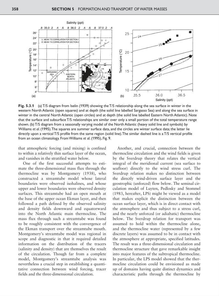
Fig. 5.3.1 (a) T/S diagram from Iselin (1939) showing the T/S relationship along the sea surface in winter in the
western North Atlantic (open squares) and at depth (the solid line labelled Sargasso Sea) and along the sea surface in
winter in the central North Atlantic (open circles) and at depth (the solid line labelled Eastern North Atlantic). Note
that the surface and subsurface T/S relationships are similar over only a small portion of the total temperature range
shown. (b) T/S diagram from a seasonally varying model of the North Atlantic (heavy solid line and symbols) by
Williams et al. (1995).The squares are summer surface data, and the circles are winter surface data; the latter lie
directly upon a vertical T/S profile from the same region (solid line).The similar dashed line is a T/S vertical profile
from an ocean climatology. From Williams et al. (1995), Fig. 9.
to within a relatively thin surface layer of the ocean,
and vanishes in the stratified water below.
One of the first successful attempts to estimate the three-dimensional mass flux through the
thermocline was by Montgomery (1938), who
constructed a streamtube model whose lateral
boundaries were observed isohalines, and whose
upper and lower boundaries were observed density
surfaces. This streamtube had an open mouth at
the base of the upper ocean Ekman layer, and then
followed a path defined by the observed salinity
and density fields downward and equatorward
into the North Atlantic main thermocline. The
mass flux through such a streamtube was found
to be roughly consistent with the convergence of
the Ekman transport over the streamtube mouth.
Montgomery’s streamtube model was regional in
scope and diagnostic in that it required detailed
information on the distribution of the tracers
(salinity and density) that are themselves the result
of the circulation. Though far from a complete
model, Montgomery’s streamtube analysis was
nevertheless a crucial step in establishing a quantitative connection between wind forcing, tracer
fields and the three-dimensional circulation.
Another, and crucial, connection between the
thermocline circulation and the wind fields is given
by the Sverdrup theory that relates the vertical
integral of the meridional current (sea surface to
seafloor) directly to the wind stress curl. The
Sverdrup relation makes no distinction between
the directly wind-driven surface layer and the
geostrophic (unforced) flow below. The seminal circulation model of Luyten, Pedlosky and Stommel
(1983, hereafter, LPS) might be viewed as a model
that makes explicit the distinction between the
ocean surface layer, which is in direct contact with
the atmosphere and thus subject to a stress curl,
and the nearly unforced (or adiabatic) thermocline
below. The Sverdrup relation for transport was
assumed to hold within the thermocline alone,
and the thermocline water (represented by a few
discrete layers) was assumed to be in contact with
the atmosphere at appropriate, specified latitudes.
The result was a three-dimensional circulation and
thermocline structure that gave remarkable insight
into major features of the subtropical thermocline.
In particular, the LPS model showed that the thermocline circulation could be envisioned as made
up of domains having quite distinct dynamics and
characteristic paths through the thermocline by
SECTION 5 FORMATION AND TRANSPORT OF WATER MASSES
358
Temperature (°C)
Temperature (°C)
Salinity (ppt)
Salinity (ppt)
(a)
(b)
.8 35.0 .2 .4 .6 .8 36.0 .2 .4 .6 .8 37.0 .2 .4
4°
6°
8°
10°
12°
14°
16°
18°
20°
22°
24°
26°
EASTERN
NORTH
ATLANTIC
SARGASSO
SEA
. MEAN T-S CORRELATION FOR SECTION 1
. MEAN T-S CORRELATION FOR SECTION 2
Fig. 5.3.1 (a) T/S diagram from Iselin (1939) showing the T/S relationship along the sea surface in winter in the
western North Atlantic (open squares) and at depth (the solid line labelled Sargasso Sea) and along the sea surface in
winter in the central North Atlantic (open circles) and at depth (the solid line labelled Eastern North Atlantic). Note
that the surface and subsurface T/S relationships are similar over only a small portion of the total temperature range
shown. (b) T/S diagram from a seasonally varying model of the North Atlantic (heavy solid line and symbols) by
Williams et al. (1995).The squares are summer surface data, and the circles are winter surface data; the latter lie
directly upon a vertical T/S profile from the same region (solid line).The similar dashed line is a T/S vertical profile
from an ocean climatology. From Williams et al. (1995), Fig. 9.