

parameterization of dispersion was inappropriate.
Eventually though, as the patch broadened still
further to scales of 300–1000 km, expression of
dispersion in terms of an apparent eddy diffusivity
was again deemed sensible, and Ledwell et al. estimated a zonal diffusivity of 2300 (1000–4000)
m
2 s
91 and a meridional diffusivity of 650 (200–
1200) m
2 s
91
. This N–S/E–W difference may reflect
strain by the mean anticyclonic gyre flow and/or
manifestation of the planetary potential vorticity
gradient restricting meridional dispersion (e.g.
Bartello and Holloway, 1991).
For completeness, we also note a special form
of lateral diffusion possible at water mass fronts:
thermohaline intrusions. Joyce (1977) discussed
how interleaving of water masses at fronts can
greatly increase the surface area and property gradients between waters and thus enhance lateral
mixing (a form of shear dispersion; Taylor, 1953).
In addition to turbulent mixing acting on the
enhanced gradients that result from vertical interleaving, intrusions also support double diffusion.
The vertical fluxes resulting from the latter may
create horizontal pressure gradients that drive
intrusions across fronts (Stern, 1967; Toole and
Georgi, 1981; McDougall, 1985a,b), giving rise to
epipycnal as well as diapycnal property fluxes.
Armi et al. (1989) discussed a beautiful ‘natural
laboratory’ study of thermohaline intrusive mixing
in which the decay of a Mediterranean water lens
was followed over 2 years. During this period,
intrusions advanced from the periphery of the lens
towards its centre at a rate of about 30 km yr
91
,
eventually reaching the core. Ruddick and Hebert
(1988) went on to infer a horizontal diffusivity for
salt due to the intrusive motions of 0.4 m
2 s
91
,
nearly as large as what Ledwell et al. derived at
their 6-month point in NATRE.
5.2.5 Diapycnal mixing in and above the
main thermocline
5.2.5.1 Ocean interior
Ocean microstructure studies conducted over the
past 30 years, chiefly sampling the main thermoclines of the North Atlantic and Pacific Oceans,
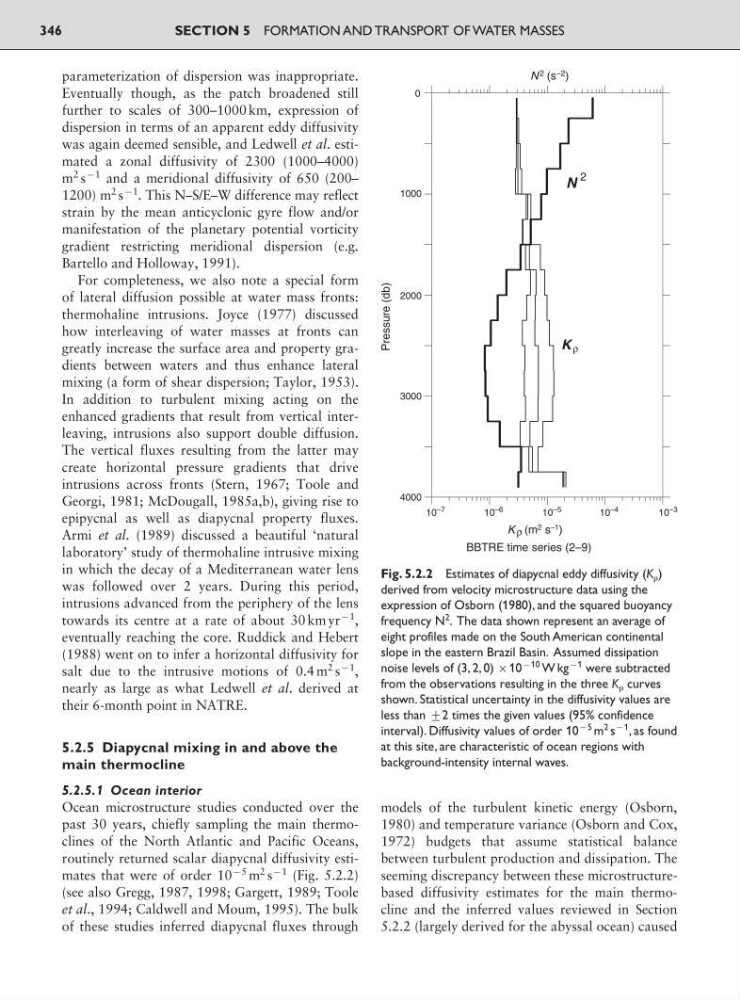
routinely returned scalar diapycnal diffusivity estimates that were of order 10
95 m
2 s
91 (Fig. 5.2.2)
(see also Gregg, 1987, 1998; Gargett, 1989; Toole
et al., 1994; Caldwell and Moum, 1995). The bulk
of these studies inferred diapycnal fluxes through
models of the turbulent kinetic energy (Osborn,
1980) and temperature variance (Osborn and Cox,
1972) budgets that assume statistical balance
between turbulent production and dissipation. The
seeming discrepancy between these microstructurebased diffusivity estimates for the main thermocline and the inferred values reviewed in Section
5.2.2 (largely derived for the abyssal ocean) caused
SECTION 5 FORMATION AND TRANSPORT OF WATER MASSES
346
0
1000
2000
3000
4000
10 –7
10 –6
10 –5
10 –4
10 –3
K (m 2 s –1 )
Pressure (db)
ρ
ρ
BBTRE time series (2–9)
K
N
2
N 2 (s –2 )
Fig. 5.2.2 Estimates of diapycnal eddy diffusivity (K )
derived from velocity microstructure data using the
expression of Osborn (1980), and the squared buoyancy
frequency N
2
. The data shown represent an average of
eight profiles made on the South American continental
slope in the eastern Brazil Basin. Assumed dissipation
noise levels of (3, 2, 0) 10
910 W kg
91 were subtracted
from the observations resulting in the three K curves
shown. Statistical uncertainty in the diffusivity values are
less than <2 times the given values (95% confidence
interval). Diffusivity values of order 10
95 m
2 s
91 , as found
at this site, are characteristic of ocean regions with
background-intensity internal waves.
Eventually though, as the patch broadened still
further to scales of 300–1000 km, expression of
dispersion in terms of an apparent eddy diffusivity
was again deemed sensible, and Ledwell et al. estimated a zonal diffusivity of 2300 (1000–4000)
m
2 s
91 and a meridional diffusivity of 650 (200–
1200) m
2 s
91
. This N–S/E–W difference may reflect
strain by the mean anticyclonic gyre flow and/or
manifestation of the planetary potential vorticity
gradient restricting meridional dispersion (e.g.
Bartello and Holloway, 1991).
For completeness, we also note a special form
of lateral diffusion possible at water mass fronts:
thermohaline intrusions. Joyce (1977) discussed
how interleaving of water masses at fronts can
greatly increase the surface area and property gradients between waters and thus enhance lateral
mixing (a form of shear dispersion; Taylor, 1953).
In addition to turbulent mixing acting on the
enhanced gradients that result from vertical interleaving, intrusions also support double diffusion.
The vertical fluxes resulting from the latter may
create horizontal pressure gradients that drive
intrusions across fronts (Stern, 1967; Toole and
Georgi, 1981; McDougall, 1985a,b), giving rise to
epipycnal as well as diapycnal property fluxes.
Armi et al. (1989) discussed a beautiful ‘natural
laboratory’ study of thermohaline intrusive mixing
in which the decay of a Mediterranean water lens
was followed over 2 years. During this period,
intrusions advanced from the periphery of the lens
towards its centre at a rate of about 30 km yr
91
,
eventually reaching the core. Ruddick and Hebert
(1988) went on to infer a horizontal diffusivity for
salt due to the intrusive motions of 0.4 m
2 s
91
,
nearly as large as what Ledwell et al. derived at
their 6-month point in NATRE.
5.2.5 Diapycnal mixing in and above the
main thermocline
5.2.5.1 Ocean interior
Ocean microstructure studies conducted over the
past 30 years, chiefly sampling the main thermoclines of the North Atlantic and Pacific Oceans,
routinely returned scalar diapycnal diffusivity estimates that were of order 10
95 m
2 s
91 (Fig. 5.2.2)
(see also Gregg, 1987, 1998; Gargett, 1989; Toole
et al., 1994; Caldwell and Moum, 1995). The bulk
of these studies inferred diapycnal fluxes through
models of the turbulent kinetic energy (Osborn,
1980) and temperature variance (Osborn and Cox,
1972) budgets that assume statistical balance
between turbulent production and dissipation. The
seeming discrepancy between these microstructurebased diffusivity estimates for the main thermocline and the inferred values reviewed in Section
5.2.2 (largely derived for the abyssal ocean) caused
SECTION 5 FORMATION AND TRANSPORT OF WATER MASSES
346
0
1000
2000
3000
4000
10 –7
10 –6
10 –5
10 –4
10 –3
K (m 2 s –1 )
Pressure (db)
ρ
ρ
BBTRE time series (2–9)
K
N
2
N 2 (s –2 )
Fig. 5.2.2 Estimates of diapycnal eddy diffusivity (K )
derived from velocity microstructure data using the
expression of Osborn (1980), and the squared buoyancy
frequency N
2
. The data shown represent an average of
eight profiles made on the South American continental
slope in the eastern Brazil Basin. Assumed dissipation
noise levels of (3, 2, 0) 10
910 W kg
91 were subtracted
from the observations resulting in the three K curves
shown. Statistical uncertainty in the diffusivity values are
less than <2 times the given values (95% confidence
interval). Diffusivity values of order 10
95 m
2 s
91 , as found
at this site, are characteristic of ocean regions with
background-intensity internal waves.