

By definition, this transport is the quasi-Stokes
streamfunction and so it must approach zero
smoothly at the top and bottom boundary, even
when the bottom boundary is sloped. Note that
this behaviour is in contrast to the theory of
Killworth (1997), which has delta functions of
transport against the top and bottom oceanic
boundaries. We believe that the physical interpretation of the quasi-Stokes streamfunction, and the
interpretation of the density of a coarse-resolution
model as being the modified density,
ϳ , precludes
these delta functions.
A Taylor series approach also shows that the
thickness-weighted horizontal velocity, V
^ , obtained
by averaging V between a pair of closely spaced
ϳ
surfaces is
V
^ ϵV
ϳ
;V
B
:V
–
;⌿ z ;O(
3
)
:V
– # ;O(
3
)
(5.2.7)
where V
ϳ is the value averaged on the density surface (that is, V
ϳ is not thickness-weighted) and
V
B
:VЈͿ
ϳzЈ z
——– is the horizontal bolus velocity due to
the correlation between the horizontal velocity
perturbations evaluated on the density surface and
the perturbations of the thickness between density
surfaces. Hence the thickness-weighted horizontal
velocity, V
^ , obtained by averaging in density coordinates, is equal to the horizontal TRM velocity,
V
– # , up to error terms of cubic order in perturbation quantities.
In a similar fashion, it can be shown that the
modified diapycnal source term, Q
– # , given by
equation (5.2.6), is equal to the thickness-weighted
source term that is obtained by averaging Q
between a pair of closely spaced
ϳ surfaces. To
date, Q
– # has been parameterized using the small
values of the diapycnal diffusivity that are observed
in the thermocline (see below). As Tandon and
Garrett (1996) have pointed out, this implies
that the eddy kinetic energy of mesoscale eddies
cannot be dissipated in the ocean interior but
rather must be dissipated near the upper and/or
lower boundaries.
When the tracer equations are examined in the
light of this TRM approach one finds that there is
only one interpretation for the tracers that are carried by eddyless coarse-resolution models: they are
the thickness-weighted mean tracer values that
would be found by averaging the tracer between
density surfaces. This dictates the way in which
ocean observations should be compared with the
output of coarse-resolution ocean models and also
the way in which ocean observations should be
averaged before performing inverse calculations.
Ocean GCM (General Circulation Model) simulations using the Gent and McWilliams (1990)
scheme have found large diapycnal transports in
the Southern Ocean for both the Eulerian-mean
flow and the quasi-Stokes circulation. Hirst and
McDougall (1998) specifically plotted the zonally
averaged streamfunctions of both the Eulerianmean flow and the quasi-Stokes flow in density
coordinates to illustrate the diapycnal nature of
both circulations (their Fig. 6). They found about
5.2 Mixing and Stirring in the Ocean Interior
343
Toole and McDougall
(a)
(b)
(c)
(d)
z R L
0
1
κ /κ 0
z
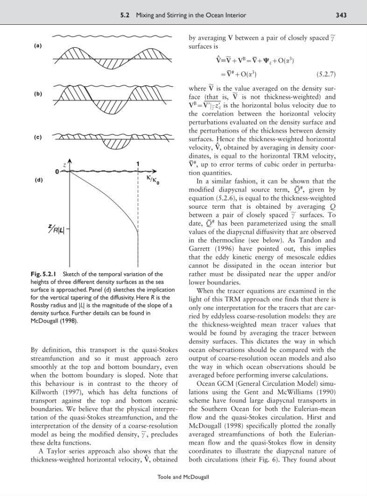
Fig. 5.2.1 Sketch of the temporal variation of the
heights of three different density surfaces as the sea
surface is approached. Panel (d) sketches the implication
for the vertical tapering of the diffusivity. Here R is the
Rossby radius and |L| is the magnitude of the slope of a
density surface. Further details can be found in
McDougall (1998).
streamfunction and so it must approach zero
smoothly at the top and bottom boundary, even
when the bottom boundary is sloped. Note that
this behaviour is in contrast to the theory of
Killworth (1997), which has delta functions of
transport against the top and bottom oceanic
boundaries. We believe that the physical interpretation of the quasi-Stokes streamfunction, and the
interpretation of the density of a coarse-resolution
model as being the modified density,
ϳ , precludes
these delta functions.
A Taylor series approach also shows that the
thickness-weighted horizontal velocity, V
^ , obtained
by averaging V between a pair of closely spaced
ϳ
surfaces is
V
^ ϵV
ϳ
;V
B
:V
–
;⌿ z ;O(
3
)
:V
– # ;O(
3
)
(5.2.7)
where V
ϳ is the value averaged on the density surface (that is, V
ϳ is not thickness-weighted) and
V
B
:VЈͿ
ϳzЈ z
——– is the horizontal bolus velocity due to
the correlation between the horizontal velocity
perturbations evaluated on the density surface and
the perturbations of the thickness between density
surfaces. Hence the thickness-weighted horizontal
velocity, V
^ , obtained by averaging in density coordinates, is equal to the horizontal TRM velocity,
V
– # , up to error terms of cubic order in perturbation quantities.
In a similar fashion, it can be shown that the
modified diapycnal source term, Q
– # , given by
equation (5.2.6), is equal to the thickness-weighted
source term that is obtained by averaging Q
between a pair of closely spaced
ϳ surfaces. To
date, Q
– # has been parameterized using the small
values of the diapycnal diffusivity that are observed
in the thermocline (see below). As Tandon and
Garrett (1996) have pointed out, this implies
that the eddy kinetic energy of mesoscale eddies
cannot be dissipated in the ocean interior but
rather must be dissipated near the upper and/or
lower boundaries.
When the tracer equations are examined in the
light of this TRM approach one finds that there is
only one interpretation for the tracers that are carried by eddyless coarse-resolution models: they are
the thickness-weighted mean tracer values that
would be found by averaging the tracer between
density surfaces. This dictates the way in which
ocean observations should be compared with the
output of coarse-resolution ocean models and also
the way in which ocean observations should be
averaged before performing inverse calculations.
Ocean GCM (General Circulation Model) simulations using the Gent and McWilliams (1990)
scheme have found large diapycnal transports in
the Southern Ocean for both the Eulerian-mean
flow and the quasi-Stokes circulation. Hirst and
McDougall (1998) specifically plotted the zonally
averaged streamfunctions of both the Eulerianmean flow and the quasi-Stokes flow in density
coordinates to illustrate the diapycnal nature of
both circulations (their Fig. 6). They found about
5.2 Mixing and Stirring in the Ocean Interior
343
Toole and McDougall
(a)
(b)
(c)
(d)
z R L
0
1
κ /κ 0
z
Fig. 5.2.1 Sketch of the temporal variation of the
heights of three different density surfaces as the sea
surface is approached. Panel (d) sketches the implication
for the vertical tapering of the diffusivity. Here R is the
Rossby radius and |L| is the magnitude of the slope of a
density surface. Further details can be found in
McDougall (1998).