

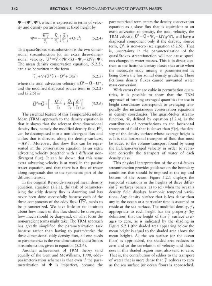
⌿:(⌿
x
, ⌿
y
), which is expressed in terms of velocity and density perturbations at fixed height by
⌿ϵ9
;
;O(
3
)
(5.2.4)
This quasi-Stokes streamfunction is the two dimensional streamfunction for an extra three-dimensional velocity, U
;
ϵ
(⌿k):⌿ z 9k(
H и⌿).
The mean density conservation equation, (5.2.2),
can also be written in the form
ϳ
t ;
и(U
– #
ϳ ):Q
– # ;O(
3 )
(5.2.5)
where the total advection velocity is
–
U
#
ϵ
–
U;U
; ,
and the modified diapycnal source term in (5.2.2)
and (5.2.5) is
Q
– # ϵQ
– ; ΄ 9 ; ΅
z
(5.2.6)
The essential feature of this Temporal-ResidualMean (TRM) approach to the density equation is
that it shows that the relevant three-dimensional
density flux, namely the modified density flux, F
M ,
can be decomposed into a non-divergent flux and
a flux that is directed along the density surfaces,
9A
ϳ . Moreover, this skew flux can be represented in the conservation equation as an extra
advecting velocity (together with a different nondivergent flux). It can be shown that this same
extra advecting velocity is at work in the passive
tracer equation, and that there is a flux of tracer
along isopycnals due to the symmetric part of the
diffusion tensor.
In the original Reynolds-averaged mean density
equation, equation (5.2.1), the task of parameterizing the eddy density flux is daunting and has
never been done successfully because each of the
three components of the eddy flux, UЈЈ
—– , needs to
be parameterized. We have little or no intuition
about how much of this flux should be divergent,
how much should be diapycnal, or what form the
non-gradient terms might take. The TRM approach
has greatly simplified the parameterization task
because rather than having to parameterize the
three-dimensional eddy density flux, all one needs
to parameterize is the two-dimensional quasi-Stokes
streamfunction, given in equation (5.2.4).
Another achievement of TRM theory (and
equally of the Gent and McWilliams, 1990, eddyparameterization scheme) is that even if the parameterization of ⌿ is imperfect, because the
parameterized term enters the density conservation
equation as a skew flux that is equivalent to an
extra advection of density, the total velocity, the
TRM velocity, U
– # :U
– ;⌿ z 9k(
H и⌿), will have a
diapycnal component only if the diabatic source
term, Q
– # , is non-zero (see equation (5.2.5)). That
is, uncertainty in the parameterization of the
quasi-Stokes streamfunction will not cause spurious changes in water masses. This is in direct contrast to the fictitious density fluxes that arise when
the mesoscale eddy mixing is parameterized as
being down the horizontal density gradient. These
fictitious density fluxes caused unwanted water
mass conversion.
With errors that are cubic in perturbation quantities, it is possible to show that the TRM
approach of forming averaged quantities for use in
height coordinates corresponds to averaging temporally the instantaneous conservation equations
in density coordinates. The quasi-Stokes streamfunction, ⌿, defined by equation (5.2.4), is the
contribution of perturbations to the horizontal
transport of fluid that is denser than
ϳ (z), the density of the density surface whose average height is
z. It is this horizontal transport of fluid that must
be added to the volume transport found by using
the Eulerian-averaged velocity in order to represent correctly the transport of water of each
density class.
This physical interpretation of the quasi-Stokes
streamfunction provides guidance on the boundary
conditions that should be imposed at the top and
bottom of the ocean. Figure 5.2.1 displays the
temporal variations in the heights of three different
ϳ surfaces (panels (a) to (c)) when the ocean’s
density field displays harmonic temporal variations. Any density surface that is less dense than
any in the ocean at a particular time is assumed to
reside at the sea surface. The modified density,
ϳ ,
appropriate to each height has the property (by
definition) that the height of this
ϳ surface averages to zero, as is indicated by the shading in
Figure 5.2.1 (the shaded area appearing below the
mean height is equal to the shaded area above the
mean height). As the sea surface (or the ocean
floor) is approached, the shaded area reduces to
zero and so the correlation of velocity and thickness in this shaded region must also tend to zero.
That is, the contribution of eddies to the transport
of water that is more dense than
ϳ reduces to zero
as the sea surface (or ocean floor) is approached.
–
ᎏ
–
z
Q
–
z
ᎏ
–
z
QЈЈ
—–
ᎏ
–
z
–
ᎏ
–
z
V
–
z
ᎏ
–
z
VЈЈ
—–
ᎏ
–
z
SECTION 5 FORMATION AND TRANSPORT OF WATER MASSES
342
x
, ⌿
y
), which is expressed in terms of velocity and density perturbations at fixed height by
⌿ϵ9
;
;O(
3
)
(5.2.4)
This quasi-Stokes streamfunction is the two dimensional streamfunction for an extra three-dimensional velocity, U
;
ϵ
(⌿k):⌿ z 9k(
H и⌿).
The mean density conservation equation, (5.2.2),
can also be written in the form
ϳ
t ;
и(U
– #
ϳ ):Q
– # ;O(
3 )
(5.2.5)
where the total advection velocity is
–
U
#
ϵ
–
U;U
; ,
and the modified diapycnal source term in (5.2.2)
and (5.2.5) is
Q
– # ϵQ
– ; ΄ 9 ; ΅
z
(5.2.6)
The essential feature of this Temporal-ResidualMean (TRM) approach to the density equation is
that it shows that the relevant three-dimensional
density flux, namely the modified density flux, F
M ,
can be decomposed into a non-divergent flux and
a flux that is directed along the density surfaces,
9A
ϳ . Moreover, this skew flux can be represented in the conservation equation as an extra
advecting velocity (together with a different nondivergent flux). It can be shown that this same
extra advecting velocity is at work in the passive
tracer equation, and that there is a flux of tracer
along isopycnals due to the symmetric part of the
diffusion tensor.
In the original Reynolds-averaged mean density
equation, equation (5.2.1), the task of parameterizing the eddy density flux is daunting and has
never been done successfully because each of the
three components of the eddy flux, UЈЈ
—– , needs to
be parameterized. We have little or no intuition
about how much of this flux should be divergent,
how much should be diapycnal, or what form the
non-gradient terms might take. The TRM approach
has greatly simplified the parameterization task
because rather than having to parameterize the
three-dimensional eddy density flux, all one needs
to parameterize is the two-dimensional quasi-Stokes
streamfunction, given in equation (5.2.4).
Another achievement of TRM theory (and
equally of the Gent and McWilliams, 1990, eddyparameterization scheme) is that even if the parameterization of ⌿ is imperfect, because the
parameterized term enters the density conservation
equation as a skew flux that is equivalent to an
extra advection of density, the total velocity, the
TRM velocity, U
– # :U
– ;⌿ z 9k(
H и⌿), will have a
diapycnal component only if the diabatic source
term, Q
– # , is non-zero (see equation (5.2.5)). That
is, uncertainty in the parameterization of the
quasi-Stokes streamfunction will not cause spurious changes in water masses. This is in direct contrast to the fictitious density fluxes that arise when
the mesoscale eddy mixing is parameterized as
being down the horizontal density gradient. These
fictitious density fluxes caused unwanted water
mass conversion.
With errors that are cubic in perturbation quantities, it is possible to show that the TRM
approach of forming averaged quantities for use in
height coordinates corresponds to averaging temporally the instantaneous conservation equations
in density coordinates. The quasi-Stokes streamfunction, ⌿, defined by equation (5.2.4), is the
contribution of perturbations to the horizontal
transport of fluid that is denser than
ϳ (z), the density of the density surface whose average height is
z. It is this horizontal transport of fluid that must
be added to the volume transport found by using
the Eulerian-averaged velocity in order to represent correctly the transport of water of each
density class.
This physical interpretation of the quasi-Stokes
streamfunction provides guidance on the boundary
conditions that should be imposed at the top and
bottom of the ocean. Figure 5.2.1 displays the
temporal variations in the heights of three different
ϳ surfaces (panels (a) to (c)) when the ocean’s
density field displays harmonic temporal variations. Any density surface that is less dense than
any in the ocean at a particular time is assumed to
reside at the sea surface. The modified density,
ϳ ,
appropriate to each height has the property (by
definition) that the height of this
ϳ surface averages to zero, as is indicated by the shading in
Figure 5.2.1 (the shaded area appearing below the
mean height is equal to the shaded area above the
mean height). As the sea surface (or the ocean
floor) is approached, the shaded area reduces to
zero and so the correlation of velocity and thickness in this shaded region must also tend to zero.
That is, the contribution of eddies to the transport
of water that is more dense than
ϳ reduces to zero
as the sea surface (or ocean floor) is approached.
–
ᎏ
–
z
Q
–
z
ᎏ
–
z
QЈЈ
—–
ᎏ
–
z
–
ᎏ
–
z
V
–
z
ᎏ
–
z
VЈЈ
—–
ᎏ
–
z
SECTION 5 FORMATION AND TRANSPORT OF WATER MASSES
342