

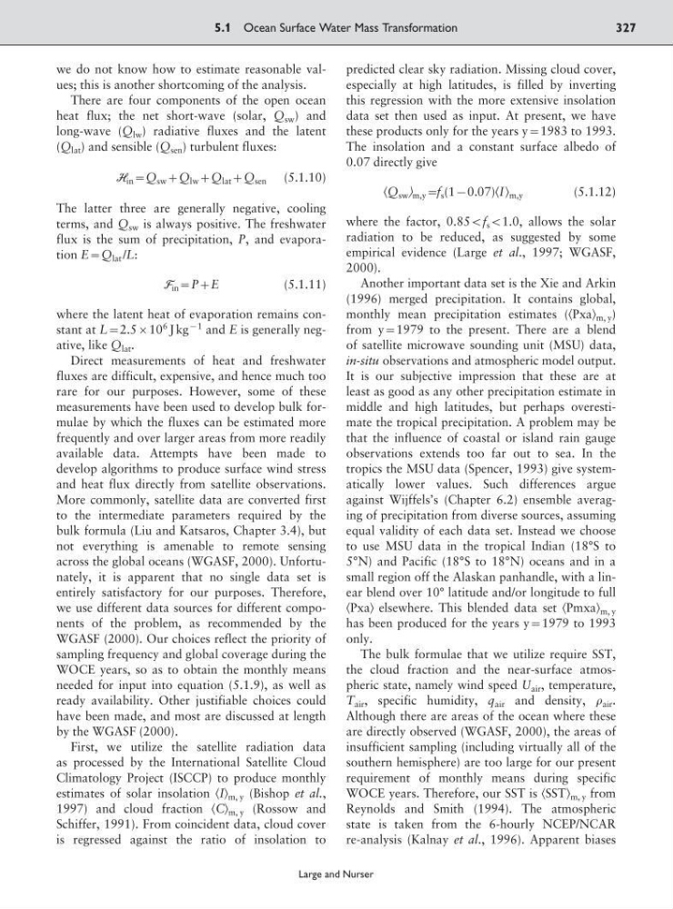
we do not know how to estimate reasonable values; this is another shortcoming of the analysis.
There are four components of the open ocean
heat flux; the net short-wave (solar, Q sw ) and
long-wave (Q lw ) radiative fluxes and the latent
(Q lat ) and sensible (Q sen ) turbulent fluxes:
H in :Q sw ;Q lw ;Q lat ;Q sen (5.1.10)
The latter three are generally negative, cooling
terms, and Q sw is always positive. The freshwater
flux is the sum of precipitation, P, and evaporation E:Q lat /L:
F in :P;E
(5.1.11)
where the latent heat of evaporation remains constant at L:2.510
6 J kg
91 and E is generally negative, like Q lat .
Direct measurements of heat and freshwater
fluxes are difficult, expensive, and hence much too
rare for our purposes. However, some of these
measurements have been used to develop bulk formulae by which the fluxes can be estimated more
frequently and over larger areas from more readily
available data. Attempts have been made to
develop algorithms to produce surface wind stress
and heat flux directly from satellite observations.
More commonly, satellite data are converted first
to the intermediate parameters required by the
bulk formula (Liu and Katsaros, Chapter 3.4), but
not everything is amenable to remote sensing
across the global oceans (WGASF, 2000). Unfortunately, it is apparent that no single data set is
entirely satisfactory for our purposes. Therefore,
we use different data sources for different components of the problem, as recommended by the
WGASF (2000). Our choices reflect the priority of
sampling frequency and global coverage during the
WOCE years, so as to obtain the monthly means
needed for input into equation (5.1.9), as well as
ready availability. Other justifiable choices could
have been made, and most are discussed at length
by the WGASF (2000).
First, we utilize the satellite radiation data
as processed by the International Satellite Cloud
Climatology Project (ISCCP) to produce monthly
estimates of solar insolation ͗I͘ m, y (Bishop et al.,
1997) and cloud fraction ͗C͘ m, y (Rossow and
Schiffer, 1991). From coincident data, cloud cover
is regressed against the ratio of insolation to
predicted clear sky radiation. Missing cloud cover,
especially at high latitudes, is filled by inverting
this regression with the more extensive insolation
data set then used as input. At present, we have
these products only for the years y:1983 to 1993.
The insolation and a constant surface albedo of
0.07 directly give
͗Q sw ͘ m,y :f s (190.07)͗I͘ m,y
(5.1.12)
where the factor, 0.85:f s :1.0, allows the solar
radiation to be reduced, as suggested by some
empirical evidence (Large et al., 1997; WGASF,
2000).
Another important data set is the Xie and Arkin
(1996) merged precipitation. It contains global,
monthly mean precipitation estimates (͗Pxa͘ m, y )
from y:1979 to the present. There are a blend
of satellite microwave sounding unit (MSU) data,
in-situ observations and atmospheric model output.
It is our subjective impression that these are at
least as good as any other precipitation estimate in
middle and high latitudes, but perhaps overestimate the tropical precipitation. A problem may be
that the influence of coastal or island rain gauge
observations extends too far out to sea. In the
tropics the MSU data (Spencer, 1993) give systematically lower values. Such differences argue
against Wijffels’s (Chapter 6.2) ensemble averaging of precipitation from diverse sources, assuming
equal validity of each data set. Instead we choose
to use MSU data in the tropical Indian (18°S to
5°N) and Pacific (18°S to 18°N) oceans and in a
small region off the Alaskan panhandle, with a linear blend over 10° latitude and/or longitude to full
͗Pxa͘ elsewhere. This blended data set ͗Pmxa͘ m, y
has been produced for the years y:1979 to 1993
only.
The bulk formulae that we utilize require SST,
the cloud fraction and the near-surface atmospheric state, namely wind speed U air , temperature,
T air , specific humidity, q air and density, air .
Although there are areas of the ocean where these
are directly observed (WGASF, 2000), the areas of
insufficient sampling (including virtually all of the
southern hemisphere) are too large for our present
requirement of monthly means during specific
WOCE years. Therefore, our SST is ͗SST͘ m, y from
Reynolds and Smith (1994). The atmospheric
state is taken from the 6-hourly NCEP/NCAR
re-analysis (Kalnay et al., 1996). Apparent biases
5.1 Ocean Surface Water Mass Transformation
327
Large and Nurser
There are four components of the open ocean
heat flux; the net short-wave (solar, Q sw ) and
long-wave (Q lw ) radiative fluxes and the latent
(Q lat ) and sensible (Q sen ) turbulent fluxes:
H in :Q sw ;Q lw ;Q lat ;Q sen (5.1.10)
The latter three are generally negative, cooling
terms, and Q sw is always positive. The freshwater
flux is the sum of precipitation, P, and evaporation E:Q lat /L:
F in :P;E
(5.1.11)
where the latent heat of evaporation remains constant at L:2.510
6 J kg
91 and E is generally negative, like Q lat .
Direct measurements of heat and freshwater
fluxes are difficult, expensive, and hence much too
rare for our purposes. However, some of these
measurements have been used to develop bulk formulae by which the fluxes can be estimated more
frequently and over larger areas from more readily
available data. Attempts have been made to
develop algorithms to produce surface wind stress
and heat flux directly from satellite observations.
More commonly, satellite data are converted first
to the intermediate parameters required by the
bulk formula (Liu and Katsaros, Chapter 3.4), but
not everything is amenable to remote sensing
across the global oceans (WGASF, 2000). Unfortunately, it is apparent that no single data set is
entirely satisfactory for our purposes. Therefore,
we use different data sources for different components of the problem, as recommended by the
WGASF (2000). Our choices reflect the priority of
sampling frequency and global coverage during the
WOCE years, so as to obtain the monthly means
needed for input into equation (5.1.9), as well as
ready availability. Other justifiable choices could
have been made, and most are discussed at length
by the WGASF (2000).
First, we utilize the satellite radiation data
as processed by the International Satellite Cloud
Climatology Project (ISCCP) to produce monthly
estimates of solar insolation ͗I͘ m, y (Bishop et al.,
1997) and cloud fraction ͗C͘ m, y (Rossow and
Schiffer, 1991). From coincident data, cloud cover
is regressed against the ratio of insolation to
predicted clear sky radiation. Missing cloud cover,
especially at high latitudes, is filled by inverting
this regression with the more extensive insolation
data set then used as input. At present, we have
these products only for the years y:1983 to 1993.
The insolation and a constant surface albedo of
0.07 directly give
͗Q sw ͘ m,y :f s (190.07)͗I͘ m,y
(5.1.12)
where the factor, 0.85:f s :1.0, allows the solar
radiation to be reduced, as suggested by some
empirical evidence (Large et al., 1997; WGASF,
2000).
Another important data set is the Xie and Arkin
(1996) merged precipitation. It contains global,
monthly mean precipitation estimates (͗Pxa͘ m, y )
from y:1979 to the present. There are a blend
of satellite microwave sounding unit (MSU) data,
in-situ observations and atmospheric model output.
It is our subjective impression that these are at
least as good as any other precipitation estimate in
middle and high latitudes, but perhaps overestimate the tropical precipitation. A problem may be
that the influence of coastal or island rain gauge
observations extends too far out to sea. In the
tropics the MSU data (Spencer, 1993) give systematically lower values. Such differences argue
against Wijffels’s (Chapter 6.2) ensemble averaging of precipitation from diverse sources, assuming
equal validity of each data set. Instead we choose
to use MSU data in the tropical Indian (18°S to
5°N) and Pacific (18°S to 18°N) oceans and in a
small region off the Alaskan panhandle, with a linear blend over 10° latitude and/or longitude to full
͗Pxa͘ elsewhere. This blended data set ͗Pmxa͘ m, y
has been produced for the years y:1979 to 1993
only.
The bulk formulae that we utilize require SST,
the cloud fraction and the near-surface atmospheric state, namely wind speed U air , temperature,
T air , specific humidity, q air and density, air .
Although there are areas of the ocean where these
are directly observed (WGASF, 2000), the areas of
insufficient sampling (including virtually all of the
southern hemisphere) are too large for our present
requirement of monthly means during specific
WOCE years. Therefore, our SST is ͗SST͘ m, y from
Reynolds and Smith (1994). The atmospheric
state is taken from the 6-hourly NCEP/NCAR
re-analysis (Kalnay et al., 1996). Apparent biases
5.1 Ocean Surface Water Mass Transformation
327
Large and Nurser