

4.2 The Interior Circulation of the Ocean
209
Webb and Suginohara
noise due to the natural variability of the current
field tends to swamp estimates of the mean currents (even after 3 years of measurements; see
Arhan et al., 1989), so other methods have to be
used.
4.2.2.3 Modern tracers in the Pacific
Better results are coming from modern tracer measurements (see Schlosser et al., Chapter 5.8), especially in the Pacific. Talley and Joyce (1992) and
Wijffels et al. (1998) have studied the tracer distribution in the deep North Pacific and shown the
existence of a series of well-defined zonal fronts
extending from 2000 m to abyssal depths (see
Fig. 4.2.2). Lupton (1998) reports on the helium
distribution in the Pacific. He shows that it forms
a series of plumes at depths near 2500 m, indicating that the currents at such depths are primarily
zonal (his main results are overlaid as arrows in
Fig. 4.2.1).
Both results give strong support to Reid’s (1997)
description of the Pacific circulation near 2500 m,
which shows a series of well-defined zonal flows.
This is markedly different from model results (i.e.
Obata et al., 1996), which show only a westward
flow with a stronger meridional circulation.
4.2.3 Theory of gyre-scale circulation
Our theoretical understanding of ocean circulation
is based primarily on the conservation laws for
mass and momentum. The momentum equation,
relative to fixed axes on a rotating earth, is,
ᎏ
Ѩ
Ѩ
u
t
ᎏ;(uиٌ)u9fu9g9ٌp;d:0
(4.2.1)
where u is velocity, t time, f the Coriolis vector, g
gravity, p pressure and d the viscous stress due to
small-scale processes.
Away from the boundaries, the ocean is
observed to be primarily geostrophic, that is to say
the main balance is between the Coriolis term and
the horizontal pressure gradient. Taking the curl
of the vertical component of equation (4.2.1), integrating it vertically, dropping small non-linear and
viscous terms and assuming that vertical velocities
are zero at depth, we obtain Sverdrup’s relation
(Sverdrup, 1947),
U y :ٌ h
(4.2.2)
U y is the north–south transport,  equals Ѩf/Ѩy and
is the surface wind stress (see Veronis, 1981;
Pedlosky, 1987b, 1996; and Müller, 1995 for
more details).
Thus away from boundaries, the north–south
transport of the ocean is zero unless there is a
wind stress curl acting locally. Additional transports can occur at boundaries, especially western
boundaries, but on the eastern boundary these are
normally observed to be small. As a result it is
possible to define a stream function that defines
the interior flow field,
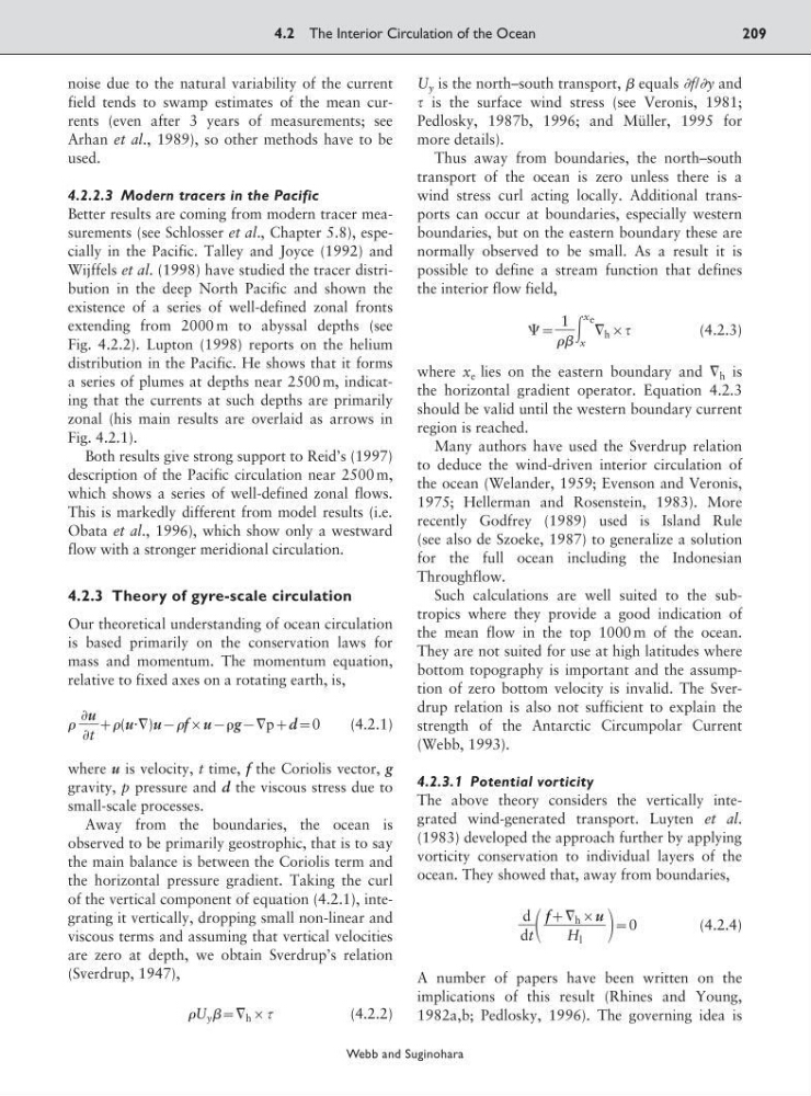
⌿:ᎏ
1

ᎏ͵
x e
x
ٌ h
(4.2.3)
where x e lies on the eastern boundary and ٌ h is
the horizontal gradient operator. Equation 4.2.3
should be valid until the western boundary current
region is reached.
Many authors have used the Sverdrup relation
to deduce the wind-driven interior circulation of
the ocean (Welander, 1959; Evenson and Veronis,
1975; Hellerman and Rosenstein, 1983). More
recently Godfrey (1989) used is Island Rule
(see also de Szoeke, 1987) to generalize a solution
for the full ocean including the Indonesian
Throughflow.
Such calculations are well suited to the subtropics where they provide a good indication of
the mean flow in the top 1000 m of the ocean.
They are not suited for use at high latitudes where
bottom topography is important and the assumption of zero bottom velocity is invalid. The Sverdrup relation is also not sufficient to explain the
strength of the Antarctic Circumpolar Current
(Webb, 1993).
4.2.3.1 Potential vorticity
The above theory considers the vertically integrated wind-generated transport. Luyten et al.
(1983) developed the approach further by applying
vorticity conservation to individual layers of the
ocean. They showed that, away from boundaries,
ᎏ
d
d
t
ᎏ
:0
(4.2.4)
A number of papers have been written on the
implications of this result (Rhines and Young,
1982a,b; Pedlosky, 1996). The governing idea is
f;ٌ h u
ᎏᎏ
H l
209
Webb and Suginohara
noise due to the natural variability of the current
field tends to swamp estimates of the mean currents (even after 3 years of measurements; see
Arhan et al., 1989), so other methods have to be
used.
4.2.2.3 Modern tracers in the Pacific
Better results are coming from modern tracer measurements (see Schlosser et al., Chapter 5.8), especially in the Pacific. Talley and Joyce (1992) and
Wijffels et al. (1998) have studied the tracer distribution in the deep North Pacific and shown the
existence of a series of well-defined zonal fronts
extending from 2000 m to abyssal depths (see
Fig. 4.2.2). Lupton (1998) reports on the helium
distribution in the Pacific. He shows that it forms
a series of plumes at depths near 2500 m, indicating that the currents at such depths are primarily
zonal (his main results are overlaid as arrows in
Fig. 4.2.1).
Both results give strong support to Reid’s (1997)
description of the Pacific circulation near 2500 m,
which shows a series of well-defined zonal flows.
This is markedly different from model results (i.e.
Obata et al., 1996), which show only a westward
flow with a stronger meridional circulation.
4.2.3 Theory of gyre-scale circulation
Our theoretical understanding of ocean circulation
is based primarily on the conservation laws for
mass and momentum. The momentum equation,
relative to fixed axes on a rotating earth, is,
ᎏ
Ѩ
Ѩ
u
t
ᎏ;(uиٌ)u9fu9g9ٌp;d:0
(4.2.1)
where u is velocity, t time, f the Coriolis vector, g
gravity, p pressure and d the viscous stress due to
small-scale processes.
Away from the boundaries, the ocean is
observed to be primarily geostrophic, that is to say
the main balance is between the Coriolis term and
the horizontal pressure gradient. Taking the curl
of the vertical component of equation (4.2.1), integrating it vertically, dropping small non-linear and
viscous terms and assuming that vertical velocities
are zero at depth, we obtain Sverdrup’s relation
(Sverdrup, 1947),
U y :ٌ h
(4.2.2)
U y is the north–south transport,  equals Ѩf/Ѩy and
is the surface wind stress (see Veronis, 1981;
Pedlosky, 1987b, 1996; and Müller, 1995 for
more details).
Thus away from boundaries, the north–south
transport of the ocean is zero unless there is a
wind stress curl acting locally. Additional transports can occur at boundaries, especially western
boundaries, but on the eastern boundary these are
normally observed to be small. As a result it is
possible to define a stream function that defines
the interior flow field,
⌿:ᎏ
1

ᎏ͵
x e
x
ٌ h
(4.2.3)
where x e lies on the eastern boundary and ٌ h is
the horizontal gradient operator. Equation 4.2.3
should be valid until the western boundary current
region is reached.
Many authors have used the Sverdrup relation
to deduce the wind-driven interior circulation of
the ocean (Welander, 1959; Evenson and Veronis,
1975; Hellerman and Rosenstein, 1983). More
recently Godfrey (1989) used is Island Rule
(see also de Szoeke, 1987) to generalize a solution
for the full ocean including the Indonesian
Throughflow.
Such calculations are well suited to the subtropics where they provide a good indication of
the mean flow in the top 1000 m of the ocean.
They are not suited for use at high latitudes where
bottom topography is important and the assumption of zero bottom velocity is invalid. The Sverdrup relation is also not sufficient to explain the
strength of the Antarctic Circumpolar Current
(Webb, 1993).
4.2.3.1 Potential vorticity
The above theory considers the vertically integrated wind-generated transport. Luyten et al.
(1983) developed the approach further by applying
vorticity conservation to individual layers of the
ocean. They showed that, away from boundaries,
ᎏ
d
d
t
ᎏ
:0
(4.2.4)
A number of papers have been written on the
implications of this result (Rhines and Young,
1982a,b; Pedlosky, 1996). The governing idea is
f;ٌ h u
ᎏᎏ
H l