

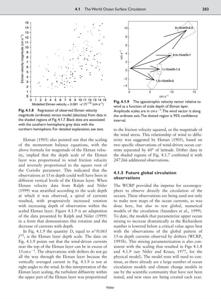
Ekman (1905) also pointed out that the scaling
of the momentum balance equations, with the
above formula for magnitude of the Ekman velocity, implied that the depth scale of the Ekman
layer was proportional to wind friction velocity
and inversely proportional to the square root of
the Coriolis parameter. This indicated that the
observations at 15 m depth could well have been in
different vertical levels of the Ekman layer. When
Ekman velocity data from Ralph and Niiler
(1999) was stratified according to the scale depth
at which it was observed, a spiral of currents
resulted, with progressively increased rotation
with increasing depth of observation within the
scaled Ekman layer. Figure 4.1.9 is an adaptation
of the data presented by Ralph and Niiler (1999)
in a form that demonstrates this rotation and the
decrease of currents with depth.
In Fig. 4.1.9 the quantity D, equal to u*/0.065
f
1/2
, is the Ekman layer depth scale. The data on
Fig. 4.1.9 points out that the wind-driven currents
near the top of the Ekman layer can be in excess of
15 cm s
91
. The observations with drifters do not go
all the way through the Ekman layer because the
vertically averaged current in Fig. 4.1.9 is not at
right angles to the wind. In this interpretation of the
Ekman layer scaling, the turbulent diffusivity within
the upper part of the Ekman layer was proportional
to the friction velocity squared, or the magnitude of
the wind stress. This relationship of wind to diffusivity was suggested by Ekman (1905), based on
two specific observations of wind-driven ocean currents separated by 60° of latitude. Drifter data in
the shaded regions of Fig. 4.1.7 confirmed it with
247 266 additional observations.
4.1.5 Future global circulation
observations
The WCRP provided the impetus for oceanographers to observe directly the circulation of the
oceans. These observations are being used not only
to make new maps of the ocean currents, as was
done here, but also to test global, numerical
models of the circulation (Saunders et al., 1999).
To date, the models that parameterize upper ocean
mixing to increase dramatically as the Richardson
number is lowered below a critical value agree best
with the observations of the global pattern of
15-m depth currents observed by drifters (WCRP,
1995b). This mixing parameterization is also consistent with the scaling that resulted in Figs 4.1.8
and 4.1.9 (see Niiler and Kraus, 1977, for the
physical model). The model tests will need to continue, as there already are a large number of ocean
circulation models and climate change models in
use by the scientific community that have not been
tested, and new ones are being created each year.
4.1 The World Ocean Surface Circulation
203
Niiler
0
1
2
3
4
5
6
7
8
9
10
11
12
13
14
15
Ekman velocity magnitude (cm s
–1
)
0 1 2 3 4 5 6 7 8 9 10 11 12 13 14 15
Modelled Ekman velocity = 0.081 u (f )
(cm s
–1 )
0
1
2
3
4
5
6
7
8
9
10
11
12
13
14
15
0 1 2 3 4 5 6 7 8 9 10 11 12 13 14 15
. *
–1/2
Fig. 4.1.8 Regression of observed Ekman velocity
magnitude (ordinate) versus model (abscissa) from data in
the shaded regions of Fig. 4.1.7. Black dots are associated
with the southern hemisphere; grey dots with the
northern hemisphere. For detailed explanation, see text.
0<15m/D<0.5
0.5<15m/D<1
1<15m/D<1.5
1.5<15m/D<2
10
8
6
4
2
0
0
–2
–4
5
1 0
1 5
cm s
–1
cm s
–1
Fig. 4.1.9 The ageostrophic velocity vector relative to
wind as a function of scale depth of Ekman layer.
Amplitude scales are in cm s
91
.The wind vector is along
the ordinate axis.The dotted region is 95% confidence
interval.
of the momentum balance equations, with the
above formula for magnitude of the Ekman velocity, implied that the depth scale of the Ekman
layer was proportional to wind friction velocity
and inversely proportional to the square root of
the Coriolis parameter. This indicated that the
observations at 15 m depth could well have been in
different vertical levels of the Ekman layer. When
Ekman velocity data from Ralph and Niiler
(1999) was stratified according to the scale depth
at which it was observed, a spiral of currents
resulted, with progressively increased rotation
with increasing depth of observation within the
scaled Ekman layer. Figure 4.1.9 is an adaptation
of the data presented by Ralph and Niiler (1999)
in a form that demonstrates this rotation and the
decrease of currents with depth.
In Fig. 4.1.9 the quantity D, equal to u*/0.065
f
1/2
, is the Ekman layer depth scale. The data on
Fig. 4.1.9 points out that the wind-driven currents
near the top of the Ekman layer can be in excess of
15 cm s
91
. The observations with drifters do not go
all the way through the Ekman layer because the
vertically averaged current in Fig. 4.1.9 is not at
right angles to the wind. In this interpretation of the
Ekman layer scaling, the turbulent diffusivity within
the upper part of the Ekman layer was proportional
to the friction velocity squared, or the magnitude of
the wind stress. This relationship of wind to diffusivity was suggested by Ekman (1905), based on
two specific observations of wind-driven ocean currents separated by 60° of latitude. Drifter data in
the shaded regions of Fig. 4.1.7 confirmed it with
247 266 additional observations.
4.1.5 Future global circulation
observations
The WCRP provided the impetus for oceanographers to observe directly the circulation of the
oceans. These observations are being used not only
to make new maps of the ocean currents, as was
done here, but also to test global, numerical
models of the circulation (Saunders et al., 1999).
To date, the models that parameterize upper ocean
mixing to increase dramatically as the Richardson
number is lowered below a critical value agree best
with the observations of the global pattern of
15-m depth currents observed by drifters (WCRP,
1995b). This mixing parameterization is also consistent with the scaling that resulted in Figs 4.1.8
and 4.1.9 (see Niiler and Kraus, 1977, for the
physical model). The model tests will need to continue, as there already are a large number of ocean
circulation models and climate change models in
use by the scientific community that have not been
tested, and new ones are being created each year.
4.1 The World Ocean Surface Circulation
203
Niiler
0
1
2
3
4
5
6
7
8
9
10
11
12
13
14
15
Ekman velocity magnitude (cm s
–1
)
0 1 2 3 4 5 6 7 8 9 10 11 12 13 14 15
Modelled Ekman velocity = 0.081 u (f )
(cm s
–1 )
0
1
2
3
4
5
6
7
8
9
10
11
12
13
14
15
0 1 2 3 4 5 6 7 8 9 10 11 12 13 14 15
. *
–1/2
Fig. 4.1.8 Regression of observed Ekman velocity
magnitude (ordinate) versus model (abscissa) from data in
the shaded regions of Fig. 4.1.7. Black dots are associated
with the southern hemisphere; grey dots with the
northern hemisphere. For detailed explanation, see text.
0<15m/D<0.5
0.5<15m/D<1
1<15m/D<1.5
1.5<15m/D<2
10
8
6
4
2
0
0
–2
–4
5
1 0
1 5
cm s
–1
cm s
–1
Fig. 4.1.9 The ageostrophic velocity vector relative to
wind as a function of scale depth of Ekman layer.
Amplitude scales are in cm s
91
.The wind vector is along
the ordinate axis.The dotted region is 95% confidence
interval.