

the Ekman layer and the nature of the turbulent
mixing coefficient within that layer.
The Ekman theory applies to wind-driven currents several degrees north or south of the equator.
To compute the Ekman currents, we used the conservation principles of momentum. At 15 m depth
observed mean velocity should be the sum of a
geostrophic velocity obtained from the pressure
gradient and a direct wind-driven velocity, the
‘Ekman velocity’ (Pedlosky, 1987b; Bi, 1995). The
15-m depth pressure gradient, and the corresponding geostrophic velocity, was computed from the
Levitus and Boyer (1994b) atlas of historical mean
temperature and salinity on a 1° latitude by 1° longitude resolution and then averaged into the same
2°6° bins used for the drifter observations. In
this latter calculation, the geostrophic velocity was
assumed to vanish at 1000 m depth. No significant
difference would result if the geostrophic velocity
were assumed to vanish at 3000 m depth. An
Ekman velocity was computed from the difference
of the total observed velocity and the geostrophic
velocity relative to 1000 m, using drifter data only
where drogues were attached.
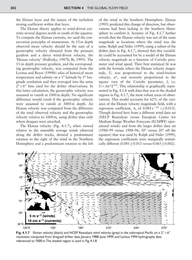
The Ekman velocity (Fig. 4.1.7), when viewed
relative to the ensemble average winds observed
along the drifter tracks, showed a predominant
rotation to the right of the wind in the Northern
Hemisphere and a predominant rotation to the left
of the wind in the Southern Hemisphere. Ekman
(1905) predicted this change of direction, but observations had been lacking in the Southern Hemisphere to confirm it. Scrutiny of Fig. 4.1.7 further
reveals that the Ekman velocity was not of the same
magnitude at locations where the wind was the
same. Ralph and Niiler (1999), using a subset of the
drifter data in Fig. 4.1.7, showed that this variability could be accounted for by a model of the Ekman
velocity magnitude as a function of Coriolis parameter and wind speed. Their best statistical fit was
with the formula where the Ekman velocity magnitude, U, was proportional to the wind-friction
velocity, u*, and inversely proportional to the
square root of the Coriolis parameter, f, i.e.
U:Au*/f
1/2
. This relationship is graphically represented in Fig. 4.1.8 with data that was in the shaded
regions in Fig. 4.1.7, the most robust areas of observations. This model accounts for 62% of the variance of the Ekman velocity magnitude field, with a
regression coefficient, A, of 0.081 s
91/2 (<0.013).
Though derived here from a different wind data set
(NECP Reanalysis versus European Centre for
Medium Range Weather Forecasts (ECMWF) operational winds) and from the larger drifter data set
(1988–99 versus 1988–96; 30° versus 20° off the
equator) that was used by Ralph and Niiler (1999),
the regression coefficients were marginally statistically different (0.081<0.013 versus 0.065<0.002).
SECTION 4 THE GLOBAL FLOW FIELD
202
30°S
20°
10°
0°
10°
20°
30°N
120°E
150°
180°
210°
240°
270°
10 cm s –1 (currents)
5 m s –1 (winds)
Fig. 4.1.7 Ekman velocity (black) and NCEP Reanalysis wind velocity (grey) in the subtropical Pacific on a 2°6°
resolution computed from drogued drifter data, January 1988–June 1999, and Levitus 1994 hydrography data
referenced to 1000 m.The shaded region is used in Fig. 4.1.8.
mixing coefficient within that layer.
The Ekman theory applies to wind-driven currents several degrees north or south of the equator.
To compute the Ekman currents, we used the conservation principles of momentum. At 15 m depth
observed mean velocity should be the sum of a
geostrophic velocity obtained from the pressure
gradient and a direct wind-driven velocity, the
‘Ekman velocity’ (Pedlosky, 1987b; Bi, 1995). The
15-m depth pressure gradient, and the corresponding geostrophic velocity, was computed from the
Levitus and Boyer (1994b) atlas of historical mean
temperature and salinity on a 1° latitude by 1° longitude resolution and then averaged into the same
2°6° bins used for the drifter observations. In
this latter calculation, the geostrophic velocity was
assumed to vanish at 1000 m depth. No significant
difference would result if the geostrophic velocity
were assumed to vanish at 3000 m depth. An
Ekman velocity was computed from the difference
of the total observed velocity and the geostrophic
velocity relative to 1000 m, using drifter data only
where drogues were attached.
The Ekman velocity (Fig. 4.1.7), when viewed
relative to the ensemble average winds observed
along the drifter tracks, showed a predominant
rotation to the right of the wind in the Northern
Hemisphere and a predominant rotation to the left
of the wind in the Southern Hemisphere. Ekman
(1905) predicted this change of direction, but observations had been lacking in the Southern Hemisphere to confirm it. Scrutiny of Fig. 4.1.7 further
reveals that the Ekman velocity was not of the same
magnitude at locations where the wind was the
same. Ralph and Niiler (1999), using a subset of the
drifter data in Fig. 4.1.7, showed that this variability could be accounted for by a model of the Ekman
velocity magnitude as a function of Coriolis parameter and wind speed. Their best statistical fit was
with the formula where the Ekman velocity magnitude, U, was proportional to the wind-friction
velocity, u*, and inversely proportional to the
square root of the Coriolis parameter, f, i.e.
U:Au*/f
1/2
. This relationship is graphically represented in Fig. 4.1.8 with data that was in the shaded
regions in Fig. 4.1.7, the most robust areas of observations. This model accounts for 62% of the variance of the Ekman velocity magnitude field, with a
regression coefficient, A, of 0.081 s
91/2 (<0.013).
Though derived here from a different wind data set
(NECP Reanalysis versus European Centre for
Medium Range Weather Forecasts (ECMWF) operational winds) and from the larger drifter data set
(1988–99 versus 1988–96; 30° versus 20° off the
equator) that was used by Ralph and Niiler (1999),
the regression coefficients were marginally statistically different (0.081<0.013 versus 0.065<0.002).
SECTION 4 THE GLOBAL FLOW FIELD
202
30°S
20°
10°
0°
10°
20°
30°N
120°E
150°
180°
210°
240°
270°
10 cm s –1 (currents)
5 m s –1 (winds)
Fig. 4.1.7 Ekman velocity (black) and NCEP Reanalysis wind velocity (grey) in the subtropical Pacific on a 2°6°
resolution computed from drogued drifter data, January 1988–June 1999, and Levitus 1994 hydrography data
referenced to 1000 m.The shaded region is used in Fig. 4.1.8.