

higher in winter than summer. A recent analysis of
4 years of T/P data indicated that these two regions
were in fact the only regions where a significant
impact of wind on the variation of eddy energy
can be determined (Stammer and Wunsch, 1999).
They suggested that the low-frequency fluctuations
of the degree of baroclinic and barotropic instabilities were important mechanisms in modulating
the eddy energy in most other regions.
Qiu (1999) discovered a pronounced annual
cycle in the eddy energy level in the Subtropical
Countercurrent in the North Pacific Ocean. This
current is located between 20°N and 25°N from
135°E to 185°E. The eddy kinetic energy in the
region reaches maximum in April–May and minimum in December–January. Using a 2.5-layer
reduced-gravity model, Qiu (1999) was able to
demonstrate that the annual variation of eddy
energy was primarily caused by the annual variation of the degree of baroclinic instability of the
Subtropical Countercurrent and the North Equatorial Current to its south. In spring the current
system has a large vertical shear and a weak vertical stratification, leading to a strong baroclinic
instability. In fall, the reverse happens and hence
the instability is reduced. The theoretical time
scale of the instability is about 60 days, matching
the observed lag of the eddy energy cycle from the
instability cycle.
Wang and Koblinsky (1999) reported that the
mesoscale sea surface height variance in the
Kuroshio Extension region varies by more than a
factor of two over 6 years based on T/P data. They
found that the temporal variation of the eddy
energy is correlated with the sea-surface-temperature difference across the Kuroshio Extension. If
the surface temperature gradient is a reflection of
the baroclinicity (or the available potential energy)
of the current, this finding is suggestive of the
baroclinic instability as a source of the eddyenergy variability.
Witter and Gordon (1999) analysed 4 years of
T/P data and discovered that the path and area
extent of the migration of the Agulhas eddies from
the Indian Ocean to the Atlantic was affected by a
basin mode of interannual variability of the South
Atlantic, which underwent a transition from a
state of enhanced gyre-scale circulation in 1993–94
to a state of weaker circulation in 1996. The
migration path of the Agulhas eddies became more
constricted and narrower in 1996 than in 1993–
94. The dynamic interpretation of the observation
is yet to be explored.
3.3.5 Concluding discussions
As discussed in Section 3.3.1, a unique aspect of
satellite altimetry is its global observation of a
dynamic boundary condition of the ocean. This
boundary condition allows inference to be made
about the circulation and density field at depths,
giving altimetric observations an important role in
providing a global perspective for integrating the
various pieces of WOCE observations to achieve a
synthetic description of the ocean circulation. A
powerful approach to achieving such a synthesis is
through the use of an ocean general circulation
model to assimilate observations for making an
estimate of the entire state of the ocean. In fact,
SECTION 3 NEW WAYS OF OBSERVING THE OCEAN
170
0
0.3
(a)
(b)
0.2
0.1
0
–0.1
–0.2
Northward heat flux (PW)
Northward salt flux (10
8
kg s
–1
)
3
2
1
0
–1
–2
60°S
6 0 °N
40°
40°
20°
20°
0°
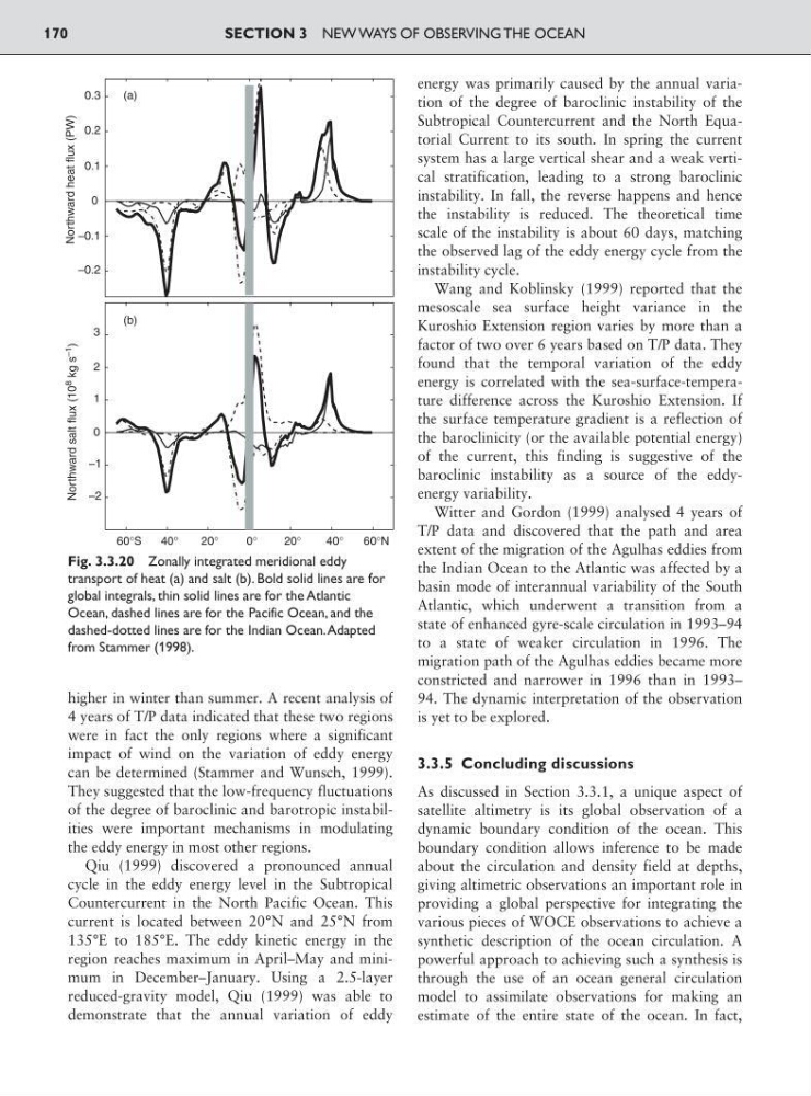
Fig. 3.3.20 Zonally integrated meridional eddy
transport of heat (a) and salt (b). Bold solid lines are for
global integrals, thin solid lines are for the Atlantic
Ocean, dashed lines are for the Pacific Ocean, and the
dashed-dotted lines are for the Indian Ocean.Adapted
from Stammer (1998).
4 years of T/P data indicated that these two regions
were in fact the only regions where a significant
impact of wind on the variation of eddy energy
can be determined (Stammer and Wunsch, 1999).
They suggested that the low-frequency fluctuations
of the degree of baroclinic and barotropic instabilities were important mechanisms in modulating
the eddy energy in most other regions.
Qiu (1999) discovered a pronounced annual
cycle in the eddy energy level in the Subtropical
Countercurrent in the North Pacific Ocean. This
current is located between 20°N and 25°N from
135°E to 185°E. The eddy kinetic energy in the
region reaches maximum in April–May and minimum in December–January. Using a 2.5-layer
reduced-gravity model, Qiu (1999) was able to
demonstrate that the annual variation of eddy
energy was primarily caused by the annual variation of the degree of baroclinic instability of the
Subtropical Countercurrent and the North Equatorial Current to its south. In spring the current
system has a large vertical shear and a weak vertical stratification, leading to a strong baroclinic
instability. In fall, the reverse happens and hence
the instability is reduced. The theoretical time
scale of the instability is about 60 days, matching
the observed lag of the eddy energy cycle from the
instability cycle.
Wang and Koblinsky (1999) reported that the
mesoscale sea surface height variance in the
Kuroshio Extension region varies by more than a
factor of two over 6 years based on T/P data. They
found that the temporal variation of the eddy
energy is correlated with the sea-surface-temperature difference across the Kuroshio Extension. If
the surface temperature gradient is a reflection of
the baroclinicity (or the available potential energy)
of the current, this finding is suggestive of the
baroclinic instability as a source of the eddyenergy variability.
Witter and Gordon (1999) analysed 4 years of
T/P data and discovered that the path and area
extent of the migration of the Agulhas eddies from
the Indian Ocean to the Atlantic was affected by a
basin mode of interannual variability of the South
Atlantic, which underwent a transition from a
state of enhanced gyre-scale circulation in 1993–94
to a state of weaker circulation in 1996. The
migration path of the Agulhas eddies became more
constricted and narrower in 1996 than in 1993–
94. The dynamic interpretation of the observation
is yet to be explored.
3.3.5 Concluding discussions
As discussed in Section 3.3.1, a unique aspect of
satellite altimetry is its global observation of a
dynamic boundary condition of the ocean. This
boundary condition allows inference to be made
about the circulation and density field at depths,
giving altimetric observations an important role in
providing a global perspective for integrating the
various pieces of WOCE observations to achieve a
synthetic description of the ocean circulation. A
powerful approach to achieving such a synthesis is
through the use of an ocean general circulation
model to assimilate observations for making an
estimate of the entire state of the ocean. In fact,
SECTION 3 NEW WAYS OF OBSERVING THE OCEAN
170
0
0.3
(a)
(b)
0.2
0.1
0
–0.1
–0.2
Northward heat flux (PW)
Northward salt flux (10
8
kg s
–1
)
3
2
1
0
–1
–2
60°S
6 0 °N
40°
40°
20°
20°
0°
Fig. 3.3.20 Zonally integrated meridional eddy
transport of heat (a) and salt (b). Bold solid lines are for
global integrals, thin solid lines are for the Atlantic
Ocean, dashed lines are for the Pacific Ocean, and the
dashed-dotted lines are for the Indian Ocean.Adapted
from Stammer (1998).