

and details of geographic pattern in comparison
with observations (Fu and Smith, 1996; Stammer
et al., 1996; McClean et al., 1997). The most
notable examples include the regions of the Gulf
Stream and Kuroshio, where the models are not
able to simulate the energetic zonal extensions of
these currents after leaving the coasts. Suspecting
that the model’s spatial resolution might be an
important factor causing these discrepancies,
Smith et al. (2000) have recently conducted a
simulation of the North Atlantic circulation at
1/10° (the previous highest resolution was 1/6°).
Comparison of this new model simulation with
combined T/P and ERS observations is shown in
Fig. 3.3.13 (see Plate 3.3.13, p. 172; after Smith
et al., 2000). The agreement represents a significant
improvement over previous simulations based on
1/6° resolution (Fu and Smith, 1996). The highest
rms variability reaches 50 cm in both the simulation and observation, whereas the previous simulation reached only 30 cm. The geographic pattern
of simulated distribution of energy has correctly
reflected the Gulf Stream extension current for the
first time. The along-track repeated observations
from T/P also allow comparison of wavenumber–
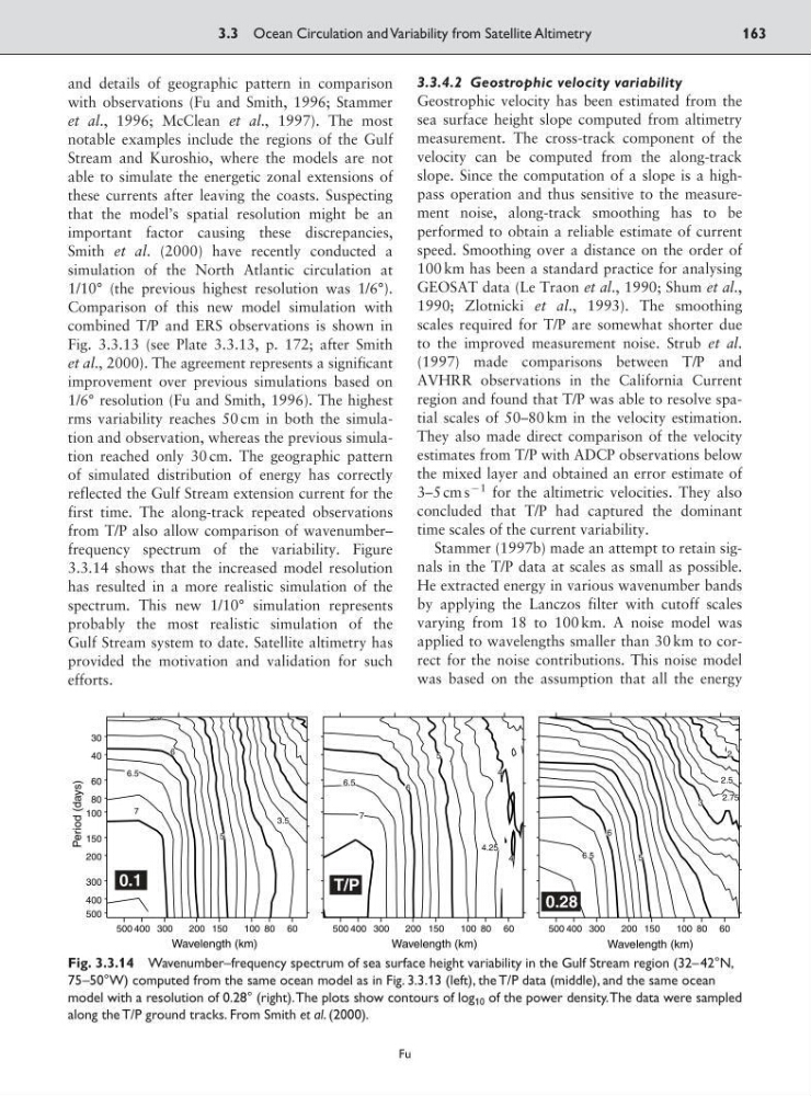
frequency spectrum of the variability. Figure
3.3.14 shows that the increased model resolution
has resulted in a more realistic simulation of the
spectrum. This new 1/10° simulation represents
probably the most realistic simulation of the
Gulf Stream system to date. Satellite altimetry has
provided the motivation and validation for such
efforts.
3.3.4.2 Geostrophic velocity variability
Geostrophic velocity has been estimated from the
sea surface height slope computed from altimetry
measurement. The cross-track component of the
velocity can be computed from the along-track
slope. Since the computation of a slope is a highpass operation and thus sensitive to the measurement noise, along-track smoothing has to be
performed to obtain a reliable estimate of current
speed. Smoothing over a distance on the order of
100 km has been a standard practice for analysing
GEOSAT data (Le Traon et al., 1990; Shum et al.,
1990; Zlotnicki et al., 1993). The smoothing
scales required for T/P are somewhat shorter due
to the improved measurement noise. Strub et al.
(1997) made comparisons between T/P and
AVHRR observations in the California Current
region and found that T/P was able to resolve spatial scales of 50–80 km in the velocity estimation.
They also made direct comparison of the velocity
estimates from T/P with ADCP observations below
the mixed layer and obtained an error estimate of
3–5 cm s
91 for the altimetric velocities. They also
concluded that T/P had captured the dominant
time scales of the current variability.
Stammer (1997b) made an attempt to retain signals in the T/P data at scales as small as possible.
He extracted energy in various wavenumber bands
by applying the Lanczos filter with cutoff scales
varying from 18 to 100 km. A noise model was
applied to wavelengths smaller than 30 km to correct for the noise contributions. This noise model
was based on the assumption that all the energy
3.3 Ocean Circulation and Variability from Satellite Altimetry
163
Fu
4
4
4.25
5
6
6.5
7
Wavelength (km)
500 400 300
200 150
100 80 60
2
2.5
2.75
3
5
6
6.5
Wavelength (km)
500 400 300
200 150
100 80 60
3.5
5
5.5
6
6.5
7
Wavelength (km)
Period (days)
500 400 300
200 150
100 80 60
500
400
300
200
150
100
80
60
40
30
0.1
T/P
0.28
Fig. 3.3.14 Wavenumber–frequency spectrum of sea surface height variability in the Gulf Stream region (32–42°N,
75–50°W) computed from the same ocean model as in Fig. 3.3.13 (left), the T/P data (middle), and the same ocean
model with a resolution of 0.28° (right).The plots show contours of log 10 of the power density.The data were sampled
along the T/P ground tracks. From Smith et al. (2000).
with observations (Fu and Smith, 1996; Stammer
et al., 1996; McClean et al., 1997). The most
notable examples include the regions of the Gulf
Stream and Kuroshio, where the models are not
able to simulate the energetic zonal extensions of
these currents after leaving the coasts. Suspecting
that the model’s spatial resolution might be an
important factor causing these discrepancies,
Smith et al. (2000) have recently conducted a
simulation of the North Atlantic circulation at
1/10° (the previous highest resolution was 1/6°).
Comparison of this new model simulation with
combined T/P and ERS observations is shown in
Fig. 3.3.13 (see Plate 3.3.13, p. 172; after Smith
et al., 2000). The agreement represents a significant
improvement over previous simulations based on
1/6° resolution (Fu and Smith, 1996). The highest
rms variability reaches 50 cm in both the simulation and observation, whereas the previous simulation reached only 30 cm. The geographic pattern
of simulated distribution of energy has correctly
reflected the Gulf Stream extension current for the
first time. The along-track repeated observations
from T/P also allow comparison of wavenumber–
frequency spectrum of the variability. Figure
3.3.14 shows that the increased model resolution
has resulted in a more realistic simulation of the
spectrum. This new 1/10° simulation represents
probably the most realistic simulation of the
Gulf Stream system to date. Satellite altimetry has
provided the motivation and validation for such
efforts.
3.3.4.2 Geostrophic velocity variability
Geostrophic velocity has been estimated from the
sea surface height slope computed from altimetry
measurement. The cross-track component of the
velocity can be computed from the along-track
slope. Since the computation of a slope is a highpass operation and thus sensitive to the measurement noise, along-track smoothing has to be
performed to obtain a reliable estimate of current
speed. Smoothing over a distance on the order of
100 km has been a standard practice for analysing
GEOSAT data (Le Traon et al., 1990; Shum et al.,
1990; Zlotnicki et al., 1993). The smoothing
scales required for T/P are somewhat shorter due
to the improved measurement noise. Strub et al.
(1997) made comparisons between T/P and
AVHRR observations in the California Current
region and found that T/P was able to resolve spatial scales of 50–80 km in the velocity estimation.
They also made direct comparison of the velocity
estimates from T/P with ADCP observations below
the mixed layer and obtained an error estimate of
3–5 cm s
91 for the altimetric velocities. They also
concluded that T/P had captured the dominant
time scales of the current variability.
Stammer (1997b) made an attempt to retain signals in the T/P data at scales as small as possible.
He extracted energy in various wavenumber bands
by applying the Lanczos filter with cutoff scales
varying from 18 to 100 km. A noise model was
applied to wavelengths smaller than 30 km to correct for the noise contributions. This noise model
was based on the assumption that all the energy
3.3 Ocean Circulation and Variability from Satellite Altimetry
163
Fu
4
4
4.25
5
6
6.5
7
Wavelength (km)
500 400 300
200 150
100 80 60
2
2.5
2.75
3
5
6
6.5
Wavelength (km)
500 400 300
200 150
100 80 60
3.5
5
5.5
6
6.5
7
Wavelength (km)
Period (days)
500 400 300
200 150
100 80 60
500
400
300
200
150
100
80
60
40
30
0.1
T/P
0.28
Fig. 3.3.14 Wavenumber–frequency spectrum of sea surface height variability in the Gulf Stream region (32–42°N,
75–50°W) computed from the same ocean model as in Fig. 3.3.13 (left), the T/P data (middle), and the same ocean
model with a resolution of 0.28° (right).The plots show contours of log 10 of the power density.The data were sampled
along the T/P ground tracks. From Smith et al. (2000).