

air/water interface, which limits the diffusion of gas
across the interface.
In aquatic systems, C surf is easily measured by gas
chromatographic analysis, and C eq may be calculated
readily if the temperature and salinity of the water
are known. In order to determine the flux of gas (F)
in or out of the water, the transfer coefficient (k)
needs to be determined. The value of k is a function
of the surface roughness of the water. In open bodies
of water, wind speed is the main determinant of
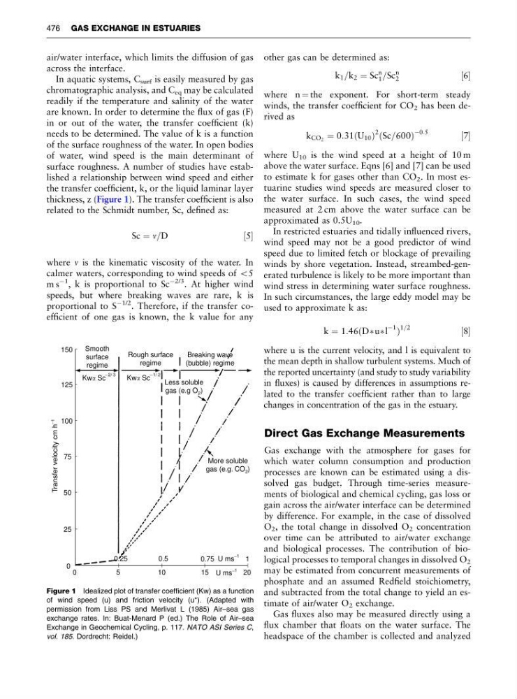
surface roughness. A number of studies have established a relationship between wind speed and either
the transfer coefficient, k, or the liquid laminar layer
thickness, z (Figure 1). The transfer coefficient is also
related to the Schmidt number, Sc, defined as:
Sc ¼ n=D
½5
where n is the kinematic viscosity of the water. In
calmer waters, corresponding to wind speeds of o5
m s
À1
, k is proportional to Sc
À2/3 . At higher wind
speeds, but where breaking waves are rare, k is
proportional to S
À1/2
. Therefore, if the transfer coefficient of one gas is known, the k value for any
other gas can be determined as:
k 1 =k 2 ¼ Sc
n
1 =Sc
n
2
½6
where n ¼ the exponent. For short-term steady
winds, the transfer coefficient for CO 2 has been derived as
k CO 2 ¼ 0:31ðU 10 Þ
2 ðSc=600Þ
À0:5
½7
where U 10 is the wind speed at a height of 10 m
above the water surface. Eqns [6] and [7] can be used
to estimate k for gases other than CO 2 . In most estuarine studies wind speeds are measured closer to
the water surface. In such cases, the wind speed
measured at 2 cm above the water surface can be
approximated as 0.5U 10 .
In restricted estuaries and tidally influenced rivers,
wind speed may not be a good predictor of wind
speed due to limited fetch or blockage of prevailing
winds by shore vegetation. Instead, streambed-generated turbulence is likely to be more important than
wind stress in determining water surface roughness.
In such circumstances, the large eddy model may be
used to approximate k as:
k ¼ 1:46ðDÃuÃl
À1 Þ
1=2
½8
where u is the current velocity, and l is equivalent to
the mean depth in shallow turbulent systems. Much of
the reported uncertainty (and study to study variability
in fluxes) is caused by differences in assumptions related to the transfer coefficient rather than to large
changes in concentration of the gas in the estuary.
Direct Gas Exchange Measurements
Gas exchange with the atmosphere for gases for
which water column consumption and production
processes are known can be estimated using a dissolved gas budget. Through time-series measurements of biological and chemical cycling, gas loss or
gain across the air/water interface can be determined
by difference. For example, in the case of dissolved
O 2 , the total change in dissolved O 2 concentration
over time can be attributed to air/water exchange
and biological processes. The contribution of biological processes to temporal changes in dissolved O 2
may be estimated from concurrent measurements of
phosphate and an assumed Redfield stoichiometry,
and subtracted from the total change to yield an estimate of air/water O 2 exchange.
Gas fluxes also may be measured directly using a
flux chamber that floats on the water surface. The
headspace of the chamber is collected and analyzed
150
125
100
75
50
25
0
0
5
10
15 U ms
_ 1
U ms
_ 1
20
1
0.75
0.5
0.25
More soluble
gas (e.g. CO )
2
Less soluble
gas (e.g O )
2
Kw Sc
_ 2/ 3
Kw Sc
_ 1/ 2
Smooth
surface
regime
Rough surface
regime
Breaking wave
(bubble) regime
Transfer velocity cm h
_
1
Figure 1 Idealized plot of transfer coefficient (Kw) as a function
of wind speed (u) and friction velocity (u*). (Adapted with
permission from Liss PS and Merlivat L (1985) Air–sea gas
exchange rates. In: Buat-Menard P (ed.) The Role of Air–sea
Exchange in Geochemical Cycling, p. 117. NATO ASI Series C,
vol. 185. Dordrecht: Reidel.)
476 GAS EXCHANGE IN ESTUARIES
across the interface.
In aquatic systems, C surf is easily measured by gas
chromatographic analysis, and C eq may be calculated
readily if the temperature and salinity of the water
are known. In order to determine the flux of gas (F)
in or out of the water, the transfer coefficient (k)
needs to be determined. The value of k is a function
of the surface roughness of the water. In open bodies
of water, wind speed is the main determinant of
surface roughness. A number of studies have established a relationship between wind speed and either
the transfer coefficient, k, or the liquid laminar layer
thickness, z (Figure 1). The transfer coefficient is also
related to the Schmidt number, Sc, defined as:
Sc ¼ n=D
½5
where n is the kinematic viscosity of the water. In
calmer waters, corresponding to wind speeds of o5
m s
À1
, k is proportional to Sc
À2/3 . At higher wind
speeds, but where breaking waves are rare, k is
proportional to S
À1/2
. Therefore, if the transfer coefficient of one gas is known, the k value for any
other gas can be determined as:
k 1 =k 2 ¼ Sc
n
1 =Sc
n
2
½6
where n ¼ the exponent. For short-term steady
winds, the transfer coefficient for CO 2 has been derived as
k CO 2 ¼ 0:31ðU 10 Þ
2 ðSc=600Þ
À0:5
½7
where U 10 is the wind speed at a height of 10 m
above the water surface. Eqns [6] and [7] can be used
to estimate k for gases other than CO 2 . In most estuarine studies wind speeds are measured closer to
the water surface. In such cases, the wind speed
measured at 2 cm above the water surface can be
approximated as 0.5U 10 .
In restricted estuaries and tidally influenced rivers,
wind speed may not be a good predictor of wind
speed due to limited fetch or blockage of prevailing
winds by shore vegetation. Instead, streambed-generated turbulence is likely to be more important than
wind stress in determining water surface roughness.
In such circumstances, the large eddy model may be
used to approximate k as:
k ¼ 1:46ðDÃuÃl
À1 Þ
1=2
½8
where u is the current velocity, and l is equivalent to
the mean depth in shallow turbulent systems. Much of
the reported uncertainty (and study to study variability
in fluxes) is caused by differences in assumptions related to the transfer coefficient rather than to large
changes in concentration of the gas in the estuary.
Direct Gas Exchange Measurements
Gas exchange with the atmosphere for gases for
which water column consumption and production
processes are known can be estimated using a dissolved gas budget. Through time-series measurements of biological and chemical cycling, gas loss or
gain across the air/water interface can be determined
by difference. For example, in the case of dissolved
O 2 , the total change in dissolved O 2 concentration
over time can be attributed to air/water exchange
and biological processes. The contribution of biological processes to temporal changes in dissolved O 2
may be estimated from concurrent measurements of
phosphate and an assumed Redfield stoichiometry,
and subtracted from the total change to yield an estimate of air/water O 2 exchange.
Gas fluxes also may be measured directly using a
flux chamber that floats on the water surface. The
headspace of the chamber is collected and analyzed
150
125
100
75
50
25
0
0
5
10
15 U ms
_ 1
U ms
_ 1
20
1
0.75
0.5
0.25
More soluble
gas (e.g. CO )
2
Less soluble
gas (e.g O )
2
Kw Sc
_ 2/ 3
Kw Sc
_ 1/ 2
Smooth
surface
regime
Rough surface
regime
Breaking wave
(bubble) regime
Transfer velocity cm h
_
1
Figure 1 Idealized plot of transfer coefficient (Kw) as a function
of wind speed (u) and friction velocity (u*). (Adapted with
permission from Liss PS and Merlivat L (1985) Air–sea gas
exchange rates. In: Buat-Menard P (ed.) The Role of Air–sea
Exchange in Geochemical Cycling, p. 117. NATO ASI Series C,
vol. 185. Dordrecht: Reidel.)
476 GAS EXCHANGE IN ESTUARIES