

early Pliocene and late Pleistocene, scientists reasoned that climatic precession and its modulation by
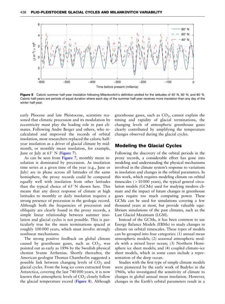
eccentricity must play the leading role in past climates. Following Andre Berger and others, who recalculated and improved the records of orbital
insolation, most researchers replaced the caloric halfyear insolation as a driver of glacial climate by midmonth, or monthly mean insolation, for example,
June or July at 651 N (Figure 7).
As can be seen from Figure 7, monthly mean insolation is dominated by precession. As insolation
time series at a given time of the year (e.g., June or
July) are in phase across all latitudes of the same
hemisphere, the proxy records could be compared
equally well with insolation from other latitudes
than the typical choice of 651 N shown here. This
means that any direct response of climate at high
latitudes to monthly or daily insolation requires a
strong presence of precession in the geologic record.
Although both the frequencies of precession and
obliquity are clearly found in the proxy records, a
simple linear relationship between summer insolation and glacial cycles is not possible. This is particularly true for the main terminations spaced at
roughly 100 000 years, which must involve strongly
nonlinear mechanisms.
The strong positive feedback on global climate
caused by greenhouse gases, such as CO 2 , was
pointed out as early as 1896 by the Swedish physical
chemist Svante Arrhenius. Shortly thereafter, the
American geologist Thomas Chamberlin suggested a
possible link between changing levels of CO 2 and
glacial cycles. From the long ice cores extracted from
Antarctica, covering the last 740 000 years, it is now
known that atmospheric levels of CO 2 closely follow
the glacial temperature record (Figure 8). Although
greenhouse gases, such as CO 2 , cannot explain the
timing and rapidity of glacial terminations, the
changing levels of atmospheric greenhouse gases
clearly contributed by amplifying the temperature
changes observed during the glacial cycles.
Modeling the Glacial Cycles
Following the discovery of the orbital periods in the
proxy records, a considerable effort has gone into
modeling and understanding the physical mechanisms
involved in the climate system’s response to variations
in insolation and changes in the orbital parameters. In
this work, which requires modeling climate on orbital
timescales (410 000 years), the typical general circulation models (GCMs) used for studying modern climate and the impact of future changes in greenhouse
gases require too much computing power. These
GCMs can be used for simulations covering a few
thousand years at most, but provide valuable equilibrium simulations of the past climates, such as the
Last Glacial Maximum (LGM).
Instead of the GCMs, it has been common to use
Energy Balance Models (EBMs) to study changes in
climate on orbital timescales. These types of models
can be grouped into four categories: (1) annual mean
atmospheric models; (2) seasonal atmospheric models with a mixed layer ocean; (3) Northern Hemisphere ice sheet models; and (4) coupled climate–ice
sheet models, which in some cases include a representation of the deep ocean.
Studies with the first type of simple climate models
were pioneered by the early work of Budyko in the
1960s, who investigated the sensitivity of climate to
changes in global annual mean insolation. However,
changes in the Earth’s orbital parameters result in a
−600
−500
−400
−300
−200
−100
0
4
2
0
2
4
6
Time before present (millenia)
(J m
−2
)
× 10
6
80° N
60° N
40° N
Figure 5 Caloric summer half-year insolation following Milankovitch’s definition plotted for the latitudes of 401 N, 601 N, and 801 N.
Caloric half-years are periods of equal duration where each day of the summer half-year receives more insolation than any day of the
winter half-year.
438 PLIO-PLEISTOCENE GLACIAL CYCLES AND MILANKOVITCH VARIABILITY
eccentricity must play the leading role in past climates. Following Andre Berger and others, who recalculated and improved the records of orbital
insolation, most researchers replaced the caloric halfyear insolation as a driver of glacial climate by midmonth, or monthly mean insolation, for example,
June or July at 651 N (Figure 7).
As can be seen from Figure 7, monthly mean insolation is dominated by precession. As insolation
time series at a given time of the year (e.g., June or
July) are in phase across all latitudes of the same
hemisphere, the proxy records could be compared
equally well with insolation from other latitudes
than the typical choice of 651 N shown here. This
means that any direct response of climate at high
latitudes to monthly or daily insolation requires a
strong presence of precession in the geologic record.
Although both the frequencies of precession and
obliquity are clearly found in the proxy records, a
simple linear relationship between summer insolation and glacial cycles is not possible. This is particularly true for the main terminations spaced at
roughly 100 000 years, which must involve strongly
nonlinear mechanisms.
The strong positive feedback on global climate
caused by greenhouse gases, such as CO 2 , was
pointed out as early as 1896 by the Swedish physical
chemist Svante Arrhenius. Shortly thereafter, the
American geologist Thomas Chamberlin suggested a
possible link between changing levels of CO 2 and
glacial cycles. From the long ice cores extracted from
Antarctica, covering the last 740 000 years, it is now
known that atmospheric levels of CO 2 closely follow
the glacial temperature record (Figure 8). Although
greenhouse gases, such as CO 2 , cannot explain the
timing and rapidity of glacial terminations, the
changing levels of atmospheric greenhouse gases
clearly contributed by amplifying the temperature
changes observed during the glacial cycles.
Modeling the Glacial Cycles
Following the discovery of the orbital periods in the
proxy records, a considerable effort has gone into
modeling and understanding the physical mechanisms
involved in the climate system’s response to variations
in insolation and changes in the orbital parameters. In
this work, which requires modeling climate on orbital
timescales (410 000 years), the typical general circulation models (GCMs) used for studying modern climate and the impact of future changes in greenhouse
gases require too much computing power. These
GCMs can be used for simulations covering a few
thousand years at most, but provide valuable equilibrium simulations of the past climates, such as the
Last Glacial Maximum (LGM).
Instead of the GCMs, it has been common to use
Energy Balance Models (EBMs) to study changes in
climate on orbital timescales. These types of models
can be grouped into four categories: (1) annual mean
atmospheric models; (2) seasonal atmospheric models with a mixed layer ocean; (3) Northern Hemisphere ice sheet models; and (4) coupled climate–ice
sheet models, which in some cases include a representation of the deep ocean.
Studies with the first type of simple climate models
were pioneered by the early work of Budyko in the
1960s, who investigated the sensitivity of climate to
changes in global annual mean insolation. However,
changes in the Earth’s orbital parameters result in a
−600
−500
−400
−300
−200
−100
0
4
2
0
2
4
6
Time before present (millenia)
(J m
−2
)
× 10
6
80° N
60° N
40° N
Figure 5 Caloric summer half-year insolation following Milankovitch’s definition plotted for the latitudes of 401 N, 601 N, and 801 N.
Caloric half-years are periods of equal duration where each day of the summer half-year receives more insolation than any day of the
winter half-year.
438 PLIO-PLEISTOCENE GLACIAL CYCLES AND MILANKOVITCH VARIABILITY