

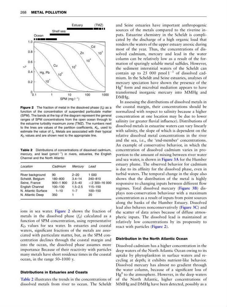
ions in sea water. Figure 2 shows the fraction of
metals in the dissolved phase (f d ) calculated as a
function of SPM concentration, using representative
K D values for sea water. In estuaries and coastal
waters, significant fractions of the metals are associated with particulate matter, but, as the SPM concentration declines through the coastal margin and
into the ocean, the dissolved phase assumes more
importance Because of their reactivity with particles
many metals have short residence times in the coastal
ocean, in the range 50–1000 y.
Distributions in Estuaries and Coasts
Table 2 illustrates the trends in the concentrations of
dissolved metals from river to ocean. The Scheldt
and Seine estuaries have important anthropogenic
sources of the metals compared to the riverine inputs. Estuarine chemistry in the Scheldt is complicated by the discharge of a high organic load that
renders the waters of the upper estuary anoxic during
most of the year. Thus, the concentrations of dissolved cadmium, mercury and lead in the water
column can be relatively low as a result of the formation of sparingly soluble metal sulfides. However,
the sediment interstitial waters of the Scheldt can
contain up to 25 000 pmol 1
À1 of dissolved cadmium. In the Scheldt and Seine estuaries, analyses of
mercury speciation have shown the presence of the
Hg
0 form and microbial mediation appears to have
transformed inorganic mercury into MMHg and
DMHg.
In assessing the distributions of dissolved metals in
the coastal margin, their concentrations should be
normalized with respect to salinity because a higher
concentration at one location may be due to lower
salinity (or greater fluvial influence). Distributions of
dissolved metals in estuarine waters can vary linearly
with salinity, the slope of which is dependent on the
relative dissolved metal concentrations in the river
and the sea, i.e., the ‘end-member’ concentrations.
An example of conservative behavior, in which the
concentration of dissolved cadmium varies in proportion to the amount of mixing between river water
and sea water, is shown in Figure 3A for the Humber
estuary plume. The observed behavior for cadmium
is due to its affinity for the dissolved phase, even in
turbid waters. The temporal change in the slope also
shows that the distribution of the metal is highly
responsive to changing inputs between different flow
regimes. Total dissolved mercury (Figure 3B) displays non-conservation behaviour with a maximum
concentration as a result of inputs from point sources
along the banks of the Humber Estuary. Dissolved
lead also behaves nonconservatively (Figure 3C) and
the scatter of data arises because of diffuse atmospheric inputs. The dissolved lead is maintained at
relatively low concentrations by its propensity to
react with particles (Figure 2).
Distribution in the North Atlantic Ocean
Dissolved cadmium has a higher concentration in the
deep waters of the North Atlantic Ocean owing to its
uptake by phytoplankton in surface waters and recycling at depth; it exhibits nutrient-like behavior.
Dissolved mercury has almost no gradient through
the water column, because of a significant loss of
Hg
0 to the atmosphere. However, in the deep waters
of the North Atlantic, higher concentrations of
MMHg and DMHg have been detected, possibly as a
Table 2 Distributions of concentrations of dissolved cadmium,
mercury, and lead (pmol l
À1 ) in rivers, estuaries, the English
Channel and the North Atlantic
Location
Cadmium
Mercury
Lead
River background
90
2–20
1 000
Scheldt, Belgium
180–800
3.4–14
240–810
Seine, France
900–1 800
2.5–40
o2 300–16 000
English Channel
100–130
1.5–2.5
115–150
N. Atlantic Surface
1–10
1–7
100–150
N. Atlantic Deep
350
1
20
1.0
0.8
0.6
0.4
0.2
0
0.1
1
10
100
1000
f d
Ocean
Shelf sea
Estuary
(TMZ)
Hg, Pb
Cu
Zn
Cd
10
7
10
6
10
5
10
4
10
3
SPM (mg l )
_ 1
Figure 2 The fraction of metal in the dissolved phase (f d ) as a
function of the concentration of suspended particulate matter
(SPM). The bands at the top of the diagram represent the general
ranges of SPM concentrations from the open ocean through to
the estuarine turbidity maximum zone (TMZ). The numbers next
to the lines are values of the partition coefficients, K D , used to
estimate the value of f d . Metals are associated with their typical
K D values and are shown next to the appropriate line.
268 METAL POLLUTION
metals in the dissolved phase (f d ) calculated as a
function of SPM concentration, using representative
K D values for sea water. In estuaries and coastal
waters, significant fractions of the metals are associated with particulate matter, but, as the SPM concentration declines through the coastal margin and
into the ocean, the dissolved phase assumes more
importance Because of their reactivity with particles
many metals have short residence times in the coastal
ocean, in the range 50–1000 y.
Distributions in Estuaries and Coasts
Table 2 illustrates the trends in the concentrations of
dissolved metals from river to ocean. The Scheldt
and Seine estuaries have important anthropogenic
sources of the metals compared to the riverine inputs. Estuarine chemistry in the Scheldt is complicated by the discharge of a high organic load that
renders the waters of the upper estuary anoxic during
most of the year. Thus, the concentrations of dissolved cadmium, mercury and lead in the water
column can be relatively low as a result of the formation of sparingly soluble metal sulfides. However,
the sediment interstitial waters of the Scheldt can
contain up to 25 000 pmol 1
À1 of dissolved cadmium. In the Scheldt and Seine estuaries, analyses of
mercury speciation have shown the presence of the
Hg
0 form and microbial mediation appears to have
transformed inorganic mercury into MMHg and
DMHg.
In assessing the distributions of dissolved metals in
the coastal margin, their concentrations should be
normalized with respect to salinity because a higher
concentration at one location may be due to lower
salinity (or greater fluvial influence). Distributions of
dissolved metals in estuarine waters can vary linearly
with salinity, the slope of which is dependent on the
relative dissolved metal concentrations in the river
and the sea, i.e., the ‘end-member’ concentrations.
An example of conservative behavior, in which the
concentration of dissolved cadmium varies in proportion to the amount of mixing between river water
and sea water, is shown in Figure 3A for the Humber
estuary plume. The observed behavior for cadmium
is due to its affinity for the dissolved phase, even in
turbid waters. The temporal change in the slope also
shows that the distribution of the metal is highly
responsive to changing inputs between different flow
regimes. Total dissolved mercury (Figure 3B) displays non-conservation behaviour with a maximum
concentration as a result of inputs from point sources
along the banks of the Humber Estuary. Dissolved
lead also behaves nonconservatively (Figure 3C) and
the scatter of data arises because of diffuse atmospheric inputs. The dissolved lead is maintained at
relatively low concentrations by its propensity to
react with particles (Figure 2).
Distribution in the North Atlantic Ocean
Dissolved cadmium has a higher concentration in the
deep waters of the North Atlantic Ocean owing to its
uptake by phytoplankton in surface waters and recycling at depth; it exhibits nutrient-like behavior.
Dissolved mercury has almost no gradient through
the water column, because of a significant loss of
Hg
0 to the atmosphere. However, in the deep waters
of the North Atlantic, higher concentrations of
MMHg and DMHg have been detected, possibly as a
Table 2 Distributions of concentrations of dissolved cadmium,
mercury, and lead (pmol l
À1 ) in rivers, estuaries, the English
Channel and the North Atlantic
Location
Cadmium
Mercury
Lead
River background
90
2–20
1 000
Scheldt, Belgium
180–800
3.4–14
240–810
Seine, France
900–1 800
2.5–40
o2 300–16 000
English Channel
100–130
1.5–2.5
115–150
N. Atlantic Surface
1–10
1–7
100–150
N. Atlantic Deep
350
1
20
1.0
0.8
0.6
0.4
0.2
0
0.1
1
10
100
1000
f d
Ocean
Shelf sea
Estuary
(TMZ)
Hg, Pb
Cu
Zn
Cd
10
7
10
6
10
5
10
4
10
3
SPM (mg l )
_ 1
Figure 2 The fraction of metal in the dissolved phase (f d ) as a
function of the concentration of suspended particulate matter
(SPM). The bands at the top of the diagram represent the general
ranges of SPM concentrations from the open ocean through to
the estuarine turbidity maximum zone (TMZ). The numbers next
to the lines are values of the partition coefficients, K D , used to
estimate the value of f d . Metals are associated with their typical
K D values and are shown next to the appropriate line.
268 METAL POLLUTION