

determination of deep ocean ventilation rates. Most of
these calculations have used a box model to approximate the ocean system. The first such estimates yielded
mean residence times for the various deep and abyssal
ocean basins of 350–900 years. Solution of these
models generally assumes a steady-state circulation,
identifiable source water regions with known D
14
C, no
mixing between water masses, and no significant biological sources or sinks. Another early approach assumed that the vertical distribution of radiocarbon in
the deep and abyssal ocean could be described by a
vertical advection–diffusion equation. This type of
calculation leads to estimates of the effect of biological
particle flux and dissolution and to the vertical upwelling and diffusion rates. The 1D vertical advection–
diffusion approach has been abandoned for 2D and
3D calculations as the available data and our knowledge of oceanic processes have increased.
When the GEOSECS data became available, box
models were again used to estimate residence times
and mass fluxes for the abyssal ocean. In this case the
model had only four boxes, one for the deep region
(41500 m) of each ocean. New bottom water formation (NADW and Antarctic Bottom Water,
AABW) were included as inputs to the Atlantic and
Circumpolar boxes. Upwelling was allowed in the
Atlantic, Pacific, and Indian boxes and exchange was
considered between the Circumpolar box and each of
the other three ocean boxes. Results from this calculation gave mean replacement times of 510, 250,
275, and 85 years for the deep Pacific, Indian, Atlantic, and Southern Ocean, respectively, and 500
years for the deep waters of the entire world.
Upwelling rates were estimated at 4–5 m y
À1 and
mass transports generally agreed with contemporary
geostrophic calculations. Applying the same
model to more recent data sets would yield the same
results.
Oxygen Utilization Rate
Radiocarbon can be used to determine the rate of
biological or geochemical processes such as the rate
at which oxygen is consumed in deep ocean water.
The simplest example of this would be the case of a
water mass moving away from a source region at a
steady rate, undergoing constant biological oxygen
uptake and not subject to mixing. In such a situation
the oxygen utilization rate could be obtained from
the slope of oxygen versus
14 C in appropriate units.
The closest approximation to this situation is the
northward transport of CDW in the abyssal Pacific,
although the mixing requirement is only approximate. Figure 12 shows such a plot for WOCE Pacific
Ocean samples from deeper than 4000 m and north
of 401S. In this case, apparent oxygen utilization
(saturated oxygen concentration at equilibration
temperature À measured oxygen concentration) rather than oxygen concentration is plotted, to remove
the effect of temperature on oxygen solubility.
The least-squares slope of 0.83 mmol kg
À1 per ppt
converts to 0.1 mmol kg
À1 y
À1 for an oxygen utilization rate. Generally, mixing with other water masses
must be accounted for prior to evaluating the gradient. With varied or additional approximations,
very similar calculations have been used to estimate
the mean formation rates of various deep water
masses.
Ocean General Circulation Model
Calibration
Oceanographic data are seldom of value for
prediction. Additionally, the effect of a changing
Depth (m)
_ 200
_ 100
0
100
2000
1000
0
Measured
PALK estimate
Silicate estimate
Depth (m)
0
50
100
150
200
2000
1000
0
PALK estimate
Silicate estimate
(A)
(B)
1500
500
1500
500
Δ
14 C (ppt)
Bomb
C (ppt)
Δ
14
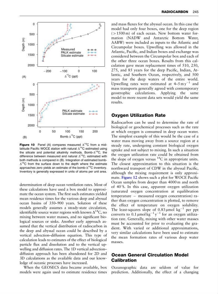
Figure 10 Panel (A) compares measured D
14 C from a midlatitude Pacific WOCE station with natural D
14 C estimated using
the silicate and potential alkalinity methods. Bomb-D
14 C, the
difference between measured and natural D
14 C, estimated with
both methods is compared in (B). Integration of estimated bombD
14 C from the surface down to the depth where the estimate
approaches zero yields an estimate of the bomb-D
14 C inventory.
Inventory is generally expressed in units of atoms per unit area.
RADIOCARBON 245
these calculations have used a box model to approximate the ocean system. The first such estimates yielded
mean residence times for the various deep and abyssal
ocean basins of 350–900 years. Solution of these
models generally assumes a steady-state circulation,
identifiable source water regions with known D
14
C, no
mixing between water masses, and no significant biological sources or sinks. Another early approach assumed that the vertical distribution of radiocarbon in
the deep and abyssal ocean could be described by a
vertical advection–diffusion equation. This type of
calculation leads to estimates of the effect of biological
particle flux and dissolution and to the vertical upwelling and diffusion rates. The 1D vertical advection–
diffusion approach has been abandoned for 2D and
3D calculations as the available data and our knowledge of oceanic processes have increased.
When the GEOSECS data became available, box
models were again used to estimate residence times
and mass fluxes for the abyssal ocean. In this case the
model had only four boxes, one for the deep region
(41500 m) of each ocean. New bottom water formation (NADW and Antarctic Bottom Water,
AABW) were included as inputs to the Atlantic and
Circumpolar boxes. Upwelling was allowed in the
Atlantic, Pacific, and Indian boxes and exchange was
considered between the Circumpolar box and each of
the other three ocean boxes. Results from this calculation gave mean replacement times of 510, 250,
275, and 85 years for the deep Pacific, Indian, Atlantic, and Southern Ocean, respectively, and 500
years for the deep waters of the entire world.
Upwelling rates were estimated at 4–5 m y
À1 and
mass transports generally agreed with contemporary
geostrophic calculations. Applying the same
model to more recent data sets would yield the same
results.
Oxygen Utilization Rate
Radiocarbon can be used to determine the rate of
biological or geochemical processes such as the rate
at which oxygen is consumed in deep ocean water.
The simplest example of this would be the case of a
water mass moving away from a source region at a
steady rate, undergoing constant biological oxygen
uptake and not subject to mixing. In such a situation
the oxygen utilization rate could be obtained from
the slope of oxygen versus
14 C in appropriate units.
The closest approximation to this situation is the
northward transport of CDW in the abyssal Pacific,
although the mixing requirement is only approximate. Figure 12 shows such a plot for WOCE Pacific
Ocean samples from deeper than 4000 m and north
of 401S. In this case, apparent oxygen utilization
(saturated oxygen concentration at equilibration
temperature À measured oxygen concentration) rather than oxygen concentration is plotted, to remove
the effect of temperature on oxygen solubility.
The least-squares slope of 0.83 mmol kg
À1 per ppt
converts to 0.1 mmol kg
À1 y
À1 for an oxygen utilization rate. Generally, mixing with other water masses
must be accounted for prior to evaluating the gradient. With varied or additional approximations,
very similar calculations have been used to estimate
the mean formation rates of various deep water
masses.
Ocean General Circulation Model
Calibration
Oceanographic data are seldom of value for
prediction. Additionally, the effect of a changing
Depth (m)
_ 200
_ 100
0
100
2000
1000
0
Measured
PALK estimate
Silicate estimate
Depth (m)
0
50
100
150
200
2000
1000
0
PALK estimate
Silicate estimate
(A)
(B)
1500
500
1500
500
Δ
14 C (ppt)
Bomb
C (ppt)
Δ
14
Figure 10 Panel (A) compares measured D
14 C from a midlatitude Pacific WOCE station with natural D
14 C estimated using
the silicate and potential alkalinity methods. Bomb-D
14 C, the
difference between measured and natural D
14 C, estimated with
both methods is compared in (B). Integration of estimated bombD
14 C from the surface down to the depth where the estimate
approaches zero yields an estimate of the bomb-D
14 C inventory.
Inventory is generally expressed in units of atoms per unit area.
RADIOCARBON 245