

Pathways of Isotopes to the Oceans
and their Approximate Inventories/
Concentrations in the Atmosphere,
Hydrosphere, and Sediments
The applications of cosmogenic isotopes as tracers
depend on three principal factors: (1) their source
function; (2) their half-lives; and (3) their chemical
properties. These considerations decide how the
fractional inventories of different tracers are distributed on the earth in the atmosphere, hydrosphere, and the sediments. The work of Lal and
Peters, using simplified models for the pathways of
the isotopes considering six mixing/exchange reservoirs is still quite instructive. These estimates of
fractional inventories of 14 isotopes amongst these
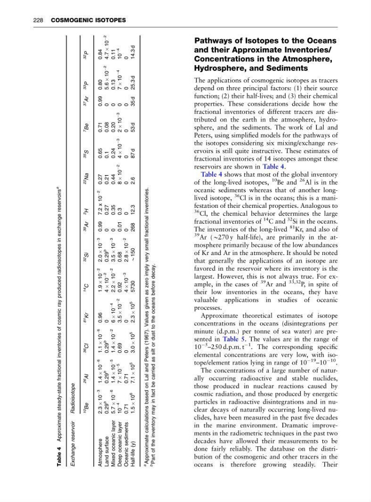
reservoirs are shown in Table 4.
Table 4 shows that most of the global inventory
of the long-lived isotopes,
10
Be and
26 Al is in the
oceanic sediments whereas that of another longlived isotope,
36
Cl is in the oceans; this is a manifestation of their chemical properties. Analogous to
36 Cl, the chemical behavior determines the large
fractional inventories of
14 C and
32 Si in the oceans.
The inventories of the long-lived
81 Kr, and also of
39 Ar (B270 y half-life), are primarily in the atmosphere primarily because of the low abundances
of Kr and Ar in the atmosphere. It should be noted
that generally the applications of an isotope are
favored in the reservoir where its inventory is the
largest. However, this is not always true. For example, in the cases of
39 Ar and
33,32 P, in spite of
their low inventories in the oceans, they have
valuable applications in studies of oceanic
processes.
Approximate theoretical estimates of isotope
concentrations in the oceans (disintegrations per
minute (d.p.m.) per tonne of sea water) are presented in Table 5. The values are in the range of
10
À5 –250 d.p.m. t
À1
. The corresponding specific
elemental concentrations are very low, with isotope/element ratios lying in range of 10
À19 –10
À10
.
The concentrations of a large number of naturally occurring radioactive and stable nuclides,
those produced in nuclear reactions caused by
cosmic radiation, and those produced by energetic
particles in radioactive disintegrations and in nuclear decays of naturally occurring long-lived nuclides, have been measured in the past five decades
in the marine environment. Dramatic improvements in the radiometric techniques in the past two
decades have allowed their measurements to be
done fairly reliably. The database on the distribution of the cosmogenic and other tracers in the
oceans is therefore growing steadily. Their
Table 4
Approximate steady-state fractional inventories of cosmic ray produced radioisotopes in exchange reservoirs
a
Exchange reservoir
Radioisotope
10
Be
26
Al
36
Cl
81
Kr
14
C
32
Si
39
Ar
3
H
22
Na
35
S
7
Be
37
Ar
33
P
32
P
Atmosphere
2.3
 10
À3
1.4
 10
À6
1.1
 10
À6
0.96
1.9
 10
À2
2.0
 10
À3
0.99 7.2 x 10
À2
0.27
0.65
0.71
0.99 0.80
0.84
Land surface
0.29
b
0.29
b
0.29
b
0
4
 10
À2
0.29
b
0
0.27
0.21
0.1
0.08
0
5.6
 10
À2
4.7
 10
À2
Mixed oceanic layer 5.7
 10
À6
1.4
 10
À5
1.4
 10
À2
6
 10
À4
2.2
 10
À2
3.5
 10
À3
0
0.35
0.44
0.24
0.20
0
0.13
0.11
Deep oceanic layer
10
À4
7
 10
À5
0.69
3.5
 10
À2
0.92
0.68
0.01 0.3
8
 10
À2
4
 10
À3
2
 10
À3
0
7Â 10
À4
10
À4
Oceanic sediments
0.71
0.71
0
0
4
 10
À3
2.8
 10
À2
0
0
0
0
0
0
0
0
Half-life (y)
1.5
 10
6
7.1
 10
5
3.0
 10
5
2.3
 10
5
5730
B150
268
12.3
2.6
87 d
53 d
35 d 25.3 d
14.3 d
a
Approximate calculations based on Lal and Peters (1967). Values given as zero imply very small fractional inventories.
b
Part of the inventory may in fact be carried as silt or dust to the oceans before decay.
228 COSMOGENIC ISOTOPES
and their Approximate Inventories/
Concentrations in the Atmosphere,
Hydrosphere, and Sediments
The applications of cosmogenic isotopes as tracers
depend on three principal factors: (1) their source
function; (2) their half-lives; and (3) their chemical
properties. These considerations decide how the
fractional inventories of different tracers are distributed on the earth in the atmosphere, hydrosphere, and the sediments. The work of Lal and
Peters, using simplified models for the pathways of
the isotopes considering six mixing/exchange reservoirs is still quite instructive. These estimates of
fractional inventories of 14 isotopes amongst these
reservoirs are shown in Table 4.
Table 4 shows that most of the global inventory
of the long-lived isotopes,
10
Be and
26 Al is in the
oceanic sediments whereas that of another longlived isotope,
36
Cl is in the oceans; this is a manifestation of their chemical properties. Analogous to
36 Cl, the chemical behavior determines the large
fractional inventories of
14 C and
32 Si in the oceans.
The inventories of the long-lived
81 Kr, and also of
39 Ar (B270 y half-life), are primarily in the atmosphere primarily because of the low abundances
of Kr and Ar in the atmosphere. It should be noted
that generally the applications of an isotope are
favored in the reservoir where its inventory is the
largest. However, this is not always true. For example, in the cases of
39 Ar and
33,32 P, in spite of
their low inventories in the oceans, they have
valuable applications in studies of oceanic
processes.
Approximate theoretical estimates of isotope
concentrations in the oceans (disintegrations per
minute (d.p.m.) per tonne of sea water) are presented in Table 5. The values are in the range of
10
À5 –250 d.p.m. t
À1
. The corresponding specific
elemental concentrations are very low, with isotope/element ratios lying in range of 10
À19 –10
À10
.
The concentrations of a large number of naturally occurring radioactive and stable nuclides,
those produced in nuclear reactions caused by
cosmic radiation, and those produced by energetic
particles in radioactive disintegrations and in nuclear decays of naturally occurring long-lived nuclides, have been measured in the past five decades
in the marine environment. Dramatic improvements in the radiometric techniques in the past two
decades have allowed their measurements to be
done fairly reliably. The database on the distribution of the cosmogenic and other tracers in the
oceans is therefore growing steadily. Their
Table 4
Approximate steady-state fractional inventories of cosmic ray produced radioisotopes in exchange reservoirs
a
Exchange reservoir
Radioisotope
10
Be
26
Al
36
Cl
81
Kr
14
C
32
Si
39
Ar
3
H
22
Na
35
S
7
Be
37
Ar
33
P
32
P
Atmosphere
2.3
 10
À3
1.4
 10
À6
1.1
 10
À6
0.96
1.9
 10
À2
2.0
 10
À3
0.99 7.2 x 10
À2
0.27
0.65
0.71
0.99 0.80
0.84
Land surface
0.29
b
0.29
b
0.29
b
0
4
 10
À2
0.29
b
0
0.27
0.21
0.1
0.08
0
5.6
 10
À2
4.7
 10
À2
Mixed oceanic layer 5.7
 10
À6
1.4
 10
À5
1.4
 10
À2
6
 10
À4
2.2
 10
À2
3.5
 10
À3
0
0.35
0.44
0.24
0.20
0
0.13
0.11
Deep oceanic layer
10
À4
7
 10
À5
0.69
3.5
 10
À2
0.92
0.68
0.01 0.3
8
 10
À2
4
 10
À3
2
 10
À3
0
7Â 10
À4
10
À4
Oceanic sediments
0.71
0.71
0
0
4
 10
À3
2.8
 10
À2
0
0
0
0
0
0
0
0
Half-life (y)
1.5
 10
6
7.1
 10
5
3.0
 10
5
2.3
 10
5
5730
B150
268
12.3
2.6
87 d
53 d
35 d 25.3 d
14.3 d
a
Approximate calculations based on Lal and Peters (1967). Values given as zero imply very small fractional inventories.
b
Part of the inventory may in fact be carried as silt or dust to the oceans before decay.
228 COSMOGENIC ISOTOPES