

to guide experiments to investigate the biology or
chemistry of an accurately marked patch of surface
water, over a period of days to weeks. Such
‘lagrangian’ experiments have frequently been performed in the past using drogued drifting buoys to
mark movement of water. However, an early observation from the trial tracer experiments made in the
English Channel was that such buoys do not normally stay co-located with a patch of water marked
by a tracer release. Surface buoys are subject to
windage and tend to slip downwind of the marked
water.
In-situ Iron Enrichment Experiments
The first use of the tracer technique to guide biogeochemical studies was in the IRONEX experiments in the equatorial Pacific. At about the time the
tracer-release technique had been developed for gasexchange experiments, the idea was suggested of
testing the ‘Iron hypothesis’ of phytoplankton limitation by releasing a large amount of iron in the
surface waters of, for example, the equatorial Pacific.
A difficulty was that if the experiment was too small,
then the iron-enriched patch would be easily lost,
whereas if it were large enough to be easily found
(probablyB100 km in scale) then it would be logistically difficult and expensive. The use of the tracer
release to guide a 10-km scale experiment was an
obvious next step, and the design for such a study
was published in 1991.
The first two unenclosed iron-enrichment studies
were carried out in 1993 and 1995 in the Equatorial
Pacific. In both, nanomolar concentrations of iron
were induced in the surface layer by release of iron
sulfate, the patches being labeled by SF 6 addition.
The SF 6 (o1 mol in total) was added in a constant
ratio to the initial addition of iron, the tracer component was then used as a guide to keep track of the
affected patch of ocean. Sampling could be reliably
categorized as ‘in’ or ‘out’ the patch, even after all
the measurable iron had disappeared from solution.
In the second study, the main experiment included
reseeding the patch with iron, but not tracer, twice
after the initial release. Important secondary aims of
the tracer component of the experiments have been
the study of mixing rates both horizontally in the
mixed layer, and vertically across the thermocline.
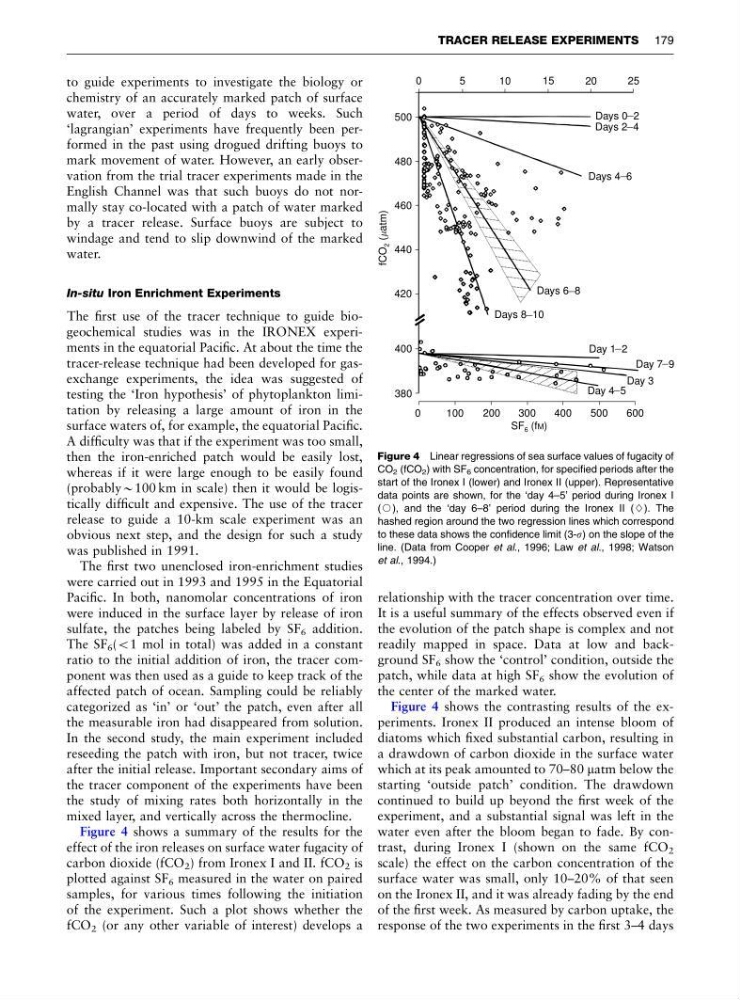
Figure 4 shows a summary of the results for the
effect of the iron releases on surface water fugacity of
carbon dioxide (fCO 2 ) from Ironex I and II. fCO 2 is
plotted against SF 6 measured in the water on paired
samples, for various times following the initiation
of the experiment. Such a plot shows whether the
fCO 2 (or any other variable of interest) develops a
relationship with the tracer concentration over time.
It is a useful summary of the effects observed even if
the evolution of the patch shape is complex and not
readily mapped in space. Data at low and background SF 6 show the ‘control’ condition, outside the
patch, while data at high SF 6 show the evolution of
the center of the marked water.
Figure 4 shows the contrasting results of the experiments. Ironex II produced an intense bloom of
diatoms which fixed substantial carbon, resulting in
a drawdown of carbon dioxide in the surface water
which at its peak amounted to 70–80 matm below the
starting ‘outside patch’ condition. The drawdown
continued to build up beyond the first week of the
experiment, and a substantial signal was left in the
water even after the bloom began to fade. By contrast, during Ironex I (shown on the same fCO 2
scale) the effect on the carbon concentration of the
surface water was small, only 10–20% of that seen
on the Ironex II, and it was already fading by the end
of the first week. As measured by carbon uptake, the
response of the two experiments in the first 3–4 days
0
5
10
500
480
460
440
420
400
380
0
100
200
300
400
500
600
SF (f )
6 M
fCO ( atm) 2
Days 6 _ 8
Days 8 _ 10
Day 4 _ 5
Day 3
Day 7 _ 9
Day 1 _ 2
Days 4 _ 6
Days 2 _ 4
Days 0 _ 2
15
20
25
Figure 4 Linear regressions of sea surface values of fugacity of
CO 2 (fCO 2 ) with SF 6 concentration, for specified periods after the
start of the Ironex I (lower) and Ironex II (upper). Representative
data points are shown, for the ‘day 4–5’ period during Ironex I
(J), and the ‘day 6–8’ period during the Ironex II (}). The
hashed region around the two regression lines which correspond
to these data shows the confidence limit (3-s) on the slope of the
line. (Data from Cooper et al., 1996; Law et al., 1998; Watson
et al., 1994.)
TRACER RELEASE EXPERIMENTS 179
chemistry of an accurately marked patch of surface
water, over a period of days to weeks. Such
‘lagrangian’ experiments have frequently been performed in the past using drogued drifting buoys to
mark movement of water. However, an early observation from the trial tracer experiments made in the
English Channel was that such buoys do not normally stay co-located with a patch of water marked
by a tracer release. Surface buoys are subject to
windage and tend to slip downwind of the marked
water.
In-situ Iron Enrichment Experiments
The first use of the tracer technique to guide biogeochemical studies was in the IRONEX experiments in the equatorial Pacific. At about the time the
tracer-release technique had been developed for gasexchange experiments, the idea was suggested of
testing the ‘Iron hypothesis’ of phytoplankton limitation by releasing a large amount of iron in the
surface waters of, for example, the equatorial Pacific.
A difficulty was that if the experiment was too small,
then the iron-enriched patch would be easily lost,
whereas if it were large enough to be easily found
(probablyB100 km in scale) then it would be logistically difficult and expensive. The use of the tracer
release to guide a 10-km scale experiment was an
obvious next step, and the design for such a study
was published in 1991.
The first two unenclosed iron-enrichment studies
were carried out in 1993 and 1995 in the Equatorial
Pacific. In both, nanomolar concentrations of iron
were induced in the surface layer by release of iron
sulfate, the patches being labeled by SF 6 addition.
The SF 6 (o1 mol in total) was added in a constant
ratio to the initial addition of iron, the tracer component was then used as a guide to keep track of the
affected patch of ocean. Sampling could be reliably
categorized as ‘in’ or ‘out’ the patch, even after all
the measurable iron had disappeared from solution.
In the second study, the main experiment included
reseeding the patch with iron, but not tracer, twice
after the initial release. Important secondary aims of
the tracer component of the experiments have been
the study of mixing rates both horizontally in the
mixed layer, and vertically across the thermocline.
Figure 4 shows a summary of the results for the
effect of the iron releases on surface water fugacity of
carbon dioxide (fCO 2 ) from Ironex I and II. fCO 2 is
plotted against SF 6 measured in the water on paired
samples, for various times following the initiation
of the experiment. Such a plot shows whether the
fCO 2 (or any other variable of interest) develops a
relationship with the tracer concentration over time.
It is a useful summary of the effects observed even if
the evolution of the patch shape is complex and not
readily mapped in space. Data at low and background SF 6 show the ‘control’ condition, outside the
patch, while data at high SF 6 show the evolution of
the center of the marked water.
Figure 4 shows the contrasting results of the experiments. Ironex II produced an intense bloom of
diatoms which fixed substantial carbon, resulting in
a drawdown of carbon dioxide in the surface water
which at its peak amounted to 70–80 matm below the
starting ‘outside patch’ condition. The drawdown
continued to build up beyond the first week of the
experiment, and a substantial signal was left in the
water even after the bloom began to fade. By contrast, during Ironex I (shown on the same fCO 2
scale) the effect on the carbon concentration of the
surface water was small, only 10–20% of that seen
on the Ironex II, and it was already fading by the end
of the first week. As measured by carbon uptake, the
response of the two experiments in the first 3–4 days
0
5
10
500
480
460
440
420
400
380
0
100
200
300
400
500
600
SF (f )
6 M
fCO ( atm) 2
Days 6 _ 8
Days 8 _ 10
Day 4 _ 5
Day 3
Day 7 _ 9
Day 1 _ 2
Days 4 _ 6
Days 2 _ 4
Days 0 _ 2
15
20
25
Figure 4 Linear regressions of sea surface values of fugacity of
CO 2 (fCO 2 ) with SF 6 concentration, for specified periods after the
start of the Ironex I (lower) and Ironex II (upper). Representative
data points are shown, for the ‘day 4–5’ period during Ironex I
(J), and the ‘day 6–8’ period during the Ironex II (}). The
hashed region around the two regression lines which correspond
to these data shows the confidence limit (3-s) on the slope of the
line. (Data from Cooper et al., 1996; Law et al., 1998; Watson
et al., 1994.)
TRACER RELEASE EXPERIMENTS 179