

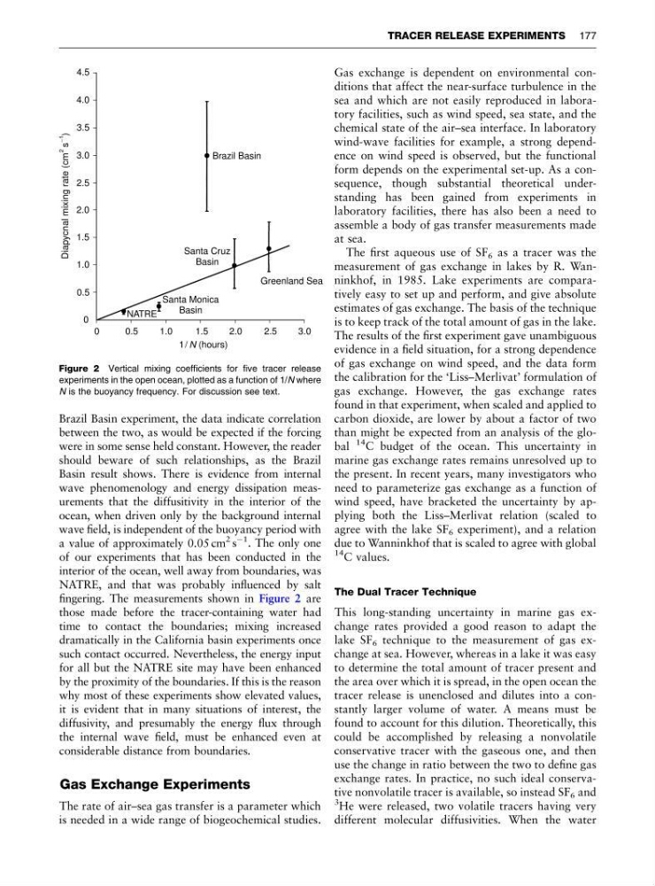
Brazil Basin experiment, the data indicate correlation
between the two, as would be expected if the forcing
were in some sense held constant. However, the reader
should beware of such relationships, as the Brazil
Basin result shows. There is evidence from internal
wave phenomenology and energy dissipation measurements that the diffusitivity in the interior of the
ocean, when driven only by the background internal
wave field, is independent of the buoyancy period with
a value of approximately 0.05 cm
2 s
À1
. The only one
of our experiments that has been conducted in the
interior of the ocean, well away from boundaries, was
NATRE, and that was probably influenced by salt
fingering. The measurements shown in Figure 2 are
those made before the tracer-containing water had
time to contact the boundaries; mixing increased
dramatically in the California basin experiments once
such contact occurred. Nevertheless, the energy input
for all but the NATRE site may have been enhanced
by the proximity of the boundaries. If this is the reason
why most of these experiments show elevated values,
it is evident that in many situations of interest, the
diffusivity, and presumably the energy flux through
the internal wave field, must be enhanced even at
considerable distance from boundaries.
Gas Exchange Experiments
The rate of air–sea gas transfer is a parameter which
is needed in a wide range of biogeochemical studies.
Gas exchange is dependent on environmental conditions that affect the near-surface turbulence in the
sea and which are not easily reproduced in laboratory facilities, such as wind speed, sea state, and the
chemical state of the air–sea interface. In laboratory
wind-wave facilities for example, a strong dependence on wind speed is observed, but the functional
form depends on the experimental set-up. As a consequence, though substantial theoretical understanding has been gained from experiments in
laboratory facilities, there has also been a need to
assemble a body of gas transfer measurements made
at sea.
The first aqueous use of SF 6 as a tracer was the
measurement of gas exchange in lakes by R. Wanninkhof, in 1985. Lake experiments are comparatively easy to set up and perform, and give absolute
estimates of gas exchange. The basis of the technique
is to keep track of the total amount of gas in the lake.
The results of the first experiment gave unambiguous
evidence in a field situation, for a strong dependence
of gas exchange on wind speed, and the data form
the calibration for the ‘Liss–Merlivat’ formulation of
gas exchange. However, the gas exchange rates
found in that experiment, when scaled and applied to
carbon dioxide, are lower by about a factor of two
than might be expected from an analysis of the global
14 C budget of the ocean. This uncertainty in
marine gas exchange rates remains unresolved up to
the present. In recent years, many investigators who
need to parameterize gas exchange as a function of
wind speed, have bracketed the uncertainty by applying both the Liss–Merlivat relation (scaled to
agree with the lake SF 6 experiment), and a relation
due to Wanninkhof that is scaled to agree with global
14 C values.
The Dual Tracer Technique
This long-standing uncertainty in marine gas exchange rates provided a good reason to adapt the
lake SF 6 technique to the measurement of gas exchange at sea. However, whereas in a lake it was easy
to determine the total amount of tracer present and
the area over which it is spread, in the open ocean the
tracer release is unenclosed and dilutes into a constantly larger volume of water. A means must be
found to account for this dilution. Theoretically, this
could be accomplished by releasing a nonvolatile
conservative tracer with the gaseous one, and then
use the change in ratio between the two to define gas
exchange rates. In practice, no such ideal conservative nonvolatile tracer is available, so instead SF 6 and
3 He were released, two volatile tracers having very
different molecular diffusivities. When the water
0
0.5
1.0
1.5
2.0
2.5
3.0
0
0.5
1.0
1.5
2.0
2.5
3.0
3.5
4.0
4.5
NATRE
Santa Monica
Basin
Santa Cruz
Basin
Greenland Sea
Brazil Basin
1/ (hours)
N
Diapycnal mixing rate (cm s )
2
_ 1
Figure 2 Vertical mixing coefficients for five tracer release
experiments in the open ocean, plotted as a function of 1/N where
N is the buoyancy frequency. For discussion see text.
TRACER RELEASE EXPERIMENTS 177
between the two, as would be expected if the forcing
were in some sense held constant. However, the reader
should beware of such relationships, as the Brazil
Basin result shows. There is evidence from internal
wave phenomenology and energy dissipation measurements that the diffusitivity in the interior of the
ocean, when driven only by the background internal
wave field, is independent of the buoyancy period with
a value of approximately 0.05 cm
2 s
À1
. The only one
of our experiments that has been conducted in the
interior of the ocean, well away from boundaries, was
NATRE, and that was probably influenced by salt
fingering. The measurements shown in Figure 2 are
those made before the tracer-containing water had
time to contact the boundaries; mixing increased
dramatically in the California basin experiments once
such contact occurred. Nevertheless, the energy input
for all but the NATRE site may have been enhanced
by the proximity of the boundaries. If this is the reason
why most of these experiments show elevated values,
it is evident that in many situations of interest, the
diffusivity, and presumably the energy flux through
the internal wave field, must be enhanced even at
considerable distance from boundaries.
Gas Exchange Experiments
The rate of air–sea gas transfer is a parameter which
is needed in a wide range of biogeochemical studies.
Gas exchange is dependent on environmental conditions that affect the near-surface turbulence in the
sea and which are not easily reproduced in laboratory facilities, such as wind speed, sea state, and the
chemical state of the air–sea interface. In laboratory
wind-wave facilities for example, a strong dependence on wind speed is observed, but the functional
form depends on the experimental set-up. As a consequence, though substantial theoretical understanding has been gained from experiments in
laboratory facilities, there has also been a need to
assemble a body of gas transfer measurements made
at sea.
The first aqueous use of SF 6 as a tracer was the
measurement of gas exchange in lakes by R. Wanninkhof, in 1985. Lake experiments are comparatively easy to set up and perform, and give absolute
estimates of gas exchange. The basis of the technique
is to keep track of the total amount of gas in the lake.
The results of the first experiment gave unambiguous
evidence in a field situation, for a strong dependence
of gas exchange on wind speed, and the data form
the calibration for the ‘Liss–Merlivat’ formulation of
gas exchange. However, the gas exchange rates
found in that experiment, when scaled and applied to
carbon dioxide, are lower by about a factor of two
than might be expected from an analysis of the global
14 C budget of the ocean. This uncertainty in
marine gas exchange rates remains unresolved up to
the present. In recent years, many investigators who
need to parameterize gas exchange as a function of
wind speed, have bracketed the uncertainty by applying both the Liss–Merlivat relation (scaled to
agree with the lake SF 6 experiment), and a relation
due to Wanninkhof that is scaled to agree with global
14 C values.
The Dual Tracer Technique
This long-standing uncertainty in marine gas exchange rates provided a good reason to adapt the
lake SF 6 technique to the measurement of gas exchange at sea. However, whereas in a lake it was easy
to determine the total amount of tracer present and
the area over which it is spread, in the open ocean the
tracer release is unenclosed and dilutes into a constantly larger volume of water. A means must be
found to account for this dilution. Theoretically, this
could be accomplished by releasing a nonvolatile
conservative tracer with the gaseous one, and then
use the change in ratio between the two to define gas
exchange rates. In practice, no such ideal conservative nonvolatile tracer is available, so instead SF 6 and
3 He were released, two volatile tracers having very
different molecular diffusivities. When the water
0
0.5
1.0
1.5
2.0
2.5
3.0
0
0.5
1.0
1.5
2.0
2.5
3.0
3.5
4.0
4.5
NATRE
Santa Monica
Basin
Santa Cruz
Basin
Greenland Sea
Brazil Basin
1/ (hours)
N
Diapycnal mixing rate (cm s )
2
_ 1
Figure 2 Vertical mixing coefficients for five tracer release
experiments in the open ocean, plotted as a function of 1/N where
N is the buoyancy frequency. For discussion see text.
TRACER RELEASE EXPERIMENTS 177